Learning Spatial Relationships with MISTy

Here, we show how to use LIANA’s implementation of MISTy, a framework presented in Tanevski et al., 2022.

MISTy is a tool that helps us better understand how different features, such as genes or cell types, interact with each other in space. MISTy does so by learning both intra- and extracellular relationships - i.e. those that occur within and between cells/spots. A major advantage of MISTy is its flexibility. It can model different perspectives, or “views,” each describing a different way markers are related to each other. Each of these views can describe a different spatial context, i.e. define a relationship among the observed expressions of the markers, such as intracellular regulation or paracrine regulation.

MISTy has only one fixed view - i.e. the intraview, which contains the target (dependent) variables. The other views we refer to as extra views, and they contain the independent variables used to predict the intra view. MISTy can fit any number of extra views, and each extra view can contain any number of variables. The extra views can thus simultaneously learn the dependencies of target variables across different modalities, such as cell type proportions, pathways, or genes, etc.

MISTy represents each view represents as a potential source of variation in the measurements of the target variables in the intra view. MISTy further analyzes each view to determine how it contributes to the overall expression or abundance of each target variable. It explains this contribution by identifying the interactions between measurements that led to the observed results.

To showcase MISTy, we use a single 10x Visium slide from Kuppe et al. (2022).

Environment

Import generic packages

import scanpy as sc
import decoupler as dc
import plotnine as p9
import liana as li

Import Helper functions needed to create MISTy objects.

from liana.method import MistyData, genericMistyData, lrMistyData

Import Pre-defined Single view models

from liana.method.sp import RandomForestModel, LinearModel, RobustLinearModel

Load and Normalize Data

We will use an ischemic 10X Visium spatial slide from Kuppe et al., 2022. It is a tissue sample obtained from a patient with myocardial infarction, specifically focusing on the ischemic zone of the heart tissue.

The slide provides spatially-resolved information about the cellular composition and gene expression patterns within the tissue.

adata = sc.read("kuppe_heart19.h5ad", backup_url='https://figshare.com/ndownloader/files/41501073?private_link=4744950f8768d5c8f68c')

adata.obs.head()

	in_tissue	array_row	array_col	sample	n_genes_by_counts	log1p_n_genes_by_counts	total_counts	log1p_total_counts	pct_counts_in_top_50_genes	pct_counts_in_top_100_genes	pct_counts_in_top_200_genes	pct_counts_in_top_500_genes	mt_frac	celltype_niche	molecular_niche
AAACAAGTATCTCCCA-1	1	50	102	Visium_19_CK297	3125	8.047510	7194.0	8.881142	24.770642	31.387267	39.797053	54.503753	0.085630	ctniche_1	molniche_9
AAACAATCTACTAGCA-1	1	3	43	Visium_19_CK297	3656	8.204398	10674.0	9.275660	35.956530	42.167885	49.456624	61.045531	0.033275	ctniche_5	molniche_3
AAACACCAATAACTGC-1	1	59	19	Visium_19_CK297	3013	8.011023	7339.0	8.901094	33.247036	39.910069	47.227143	59.326884	0.029139	ctniche_5	molniche_3
AAACAGAGCGACTCCT-1	1	14	94	Visium_19_CK297	4774	8.471149	14235.0	9.563529	22.739726	29.884089	37.850369	51.099403	0.149194	ctniche_7	molniche_2
AAACAGCTTTCAGAAG-1	1	43	9	Visium_19_CK297	2734	7.913887	6920.0	8.842316	35.664740	42.268786	50.000000	62.384393	0.025601	ctniche_5	molniche_3

Normalize data

adata.layers['counts'] = adata.X.copy()
sc.pp.normalize_total(adata, target_sum=1e4)
sc.pp.log1p(adata)

Spot clusters

sc.pl.spatial(adata, color=[None, 'celltype_niche'], size=1.3, palette='Set1')

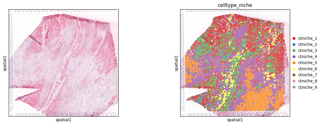
Extract Cell type Composition

This slide comes with estimated cell type proportions using cell2location; See Kuppe et al., 2022. Let’s extract from .obsm them to an independent AnnData object.

# Rename to more informative names
full_names = {'Adipo': 'Adipocytes',
              'CM': 'Cardiomyocytes',
              'Endo': 'Endothelial',
              'Fib': 'Fibroblasts',
              'PC': 'Pericytes',
              'prolif': 'Proliferating',
              'vSMCs': 'Vascular_SMCs',
              }
# but only for the ones that are in the data
adata.obsm['compositions'].columns = [full_names.get(c, c) for c in adata.obsm['compositions'].columns]

comps = li.ut.obsm_to_adata(adata, 'compositions')

comps.var

Adipocytes
Cardiomyocytes
Endothelial
Fibroblasts
Lymphoid
Mast
Myeloid
Neuronal
Pericytes
Proliferating
Vascular_SMCs

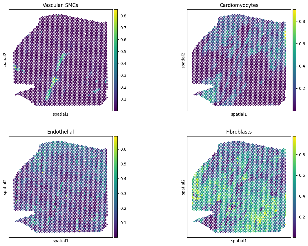
# check key cell types
sc.pl.spatial(comps,
              color=['Vascular_SMCs','Cardiomyocytes',
                     'Endothelial', 'Fibroblasts'],
              size=1.3, ncols=2, alpha_img=0
              )

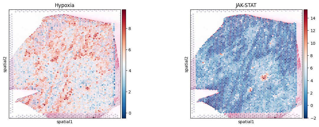
Funcomics

Before we run MISTy, let’s estimate pathway activities as a way to make the data a bit more interpretable. We will use decoupler-py with pathways genesets from PROGENy. See this tutorial for details.

# obtain genesets
progeny = dc.op.progeny(organism='human', top=500)

# use multivariate linear model to estimate activity
dc.mt.mlm(
    adata,
    net=progeny,
    verbose=True,
    raw=False
)

# extract progeny activities as an AnnData object
acts_progeny = li.ut.obsm_to_adata(adata, 'score_mlm')

# Check how the pathway activities look like
sc.pl.spatial(acts_progeny, color=['Hypoxia', 'JAK-STAT'], cmap='RdBu_r', size=1.3)

Formatting & Running MISTy

The implementation of MISTy in LIANA relies on MuData objects (Bredikhin et al., 2022) and extends them to a very simple child class we call “MistyData”. To make it easier to use, we provide functions to construct “MistyData” objects that transform the data into a format that MISTy can use.

Briefly, a “MistyData” object is just a MuData object with intra as one of the modalities - this is the view in which the (target) variables explained by all other views are stored. MISTy is flexible to any other view that is appended, provided it also contains a spatial neighbors graph.

Writing a MistyData object will simply result in a MuData object being written to disk. To read it back as MistyData, use `mudata.read_h5ad` and pass back it to the `MistyData()` function.

Let’s use genericMistyData to construct a MuData object with the intra view and the cell type proportions as the first view. Then it additionally build a ‘juxta’ view for the spots that are neighbors of each other, and a ‘para’ view for all surrounding spots within a certain radius, or bandwidth.

In this case, we will use cell type compositions per spot as the intra view, and we will use the PROGENy pathway activities as the juxta and para views:

misty = genericMistyData(intra=comps, extra=acts_progeny, cutoff=0.05, bandwidth=200, n_neighs=6)

misty

MuData object with n_obs × n_vars = 4113 × 39
  obs:	'in_tissue', 'array_row', 'array_col', 'sample', 'n_genes_by_counts', 'log1p_n_genes_by_counts', 'total_counts', 'log1p_total_counts', 'pct_counts_in_top_50_genes', 'pct_counts_in_top_100_genes', 'pct_counts_in_top_200_genes', 'pct_counts_in_top_500_genes', 'mt_frac', 'celltype_niche', 'molecular_niche'
  3 modalities
    intra:	4113 x 11
      obs:	'in_tissue', 'array_row', 'array_col', 'sample', 'n_genes_by_counts', 'log1p_n_genes_by_counts', 'total_counts', 'log1p_total_counts', 'pct_counts_in_top_50_genes', 'pct_counts_in_top_100_genes', 'pct_counts_in_top_200_genes', 'pct_counts_in_top_500_genes', 'mt_frac', 'celltype_niche', 'molecular_niche'
      obsm:	'spatial'
    juxta:	4113 x 14
      obsm:	'spatial'
      layers:	'weighted'
      obsp:	'spatial_connectivities'
    para:	4113 x 14
      obsm:	'spatial'
      layers:	'weighted'
      obsp:	'spatial_connectivities'

Learn Relationships with MISTy

Now that we have constructed the object, let’s learn the relationships across the views.

misty(model=RandomForestModel, n_jobs=-1, verbose = True)

Specifically, we will use the RandomForestModel to fit an individual random forrest model for each target in the intra view, using the juxta and para views as predictors.

MISTy returns two DataFrames:

• target_metrics - the metrics that describe the target variables from the intra view, including R-squared across different views as well as the estimated contributions to the predictive performance of each view per target.

• interactions - feature importances per view

if inplace is true (Default), these are appended to the MuData object.

Let’s check the variance explained when predicting each target variables in the intra view, with other variables (predictors) in the intra view itself. We can see that it explains itself relatively well (as expected).

misty.uns['target_metrics'].head()

	target	intra_R2	multi_R2	gain_R2	intra	juxta	para
0	Adipocytes	0.214792	0.274440	0.059648	0.509325	0.256886	0.233789
1	Cardiomyocytes	0.877458	0.892889	0.015430	0.780809	0.031148	0.188043
2	Endothelial	0.739934	0.740134	0.000200	0.946164	0.000000	0.053836
3	Fibroblasts	0.934693	0.934840	0.000147	0.968578	0.007990	0.023432
4	Lymphoid	0.101252	0.127694	0.026441	0.566420	0.125057	0.308523

li.pl.target_metrics(misty, stat='intra_R2', return_fig=True)

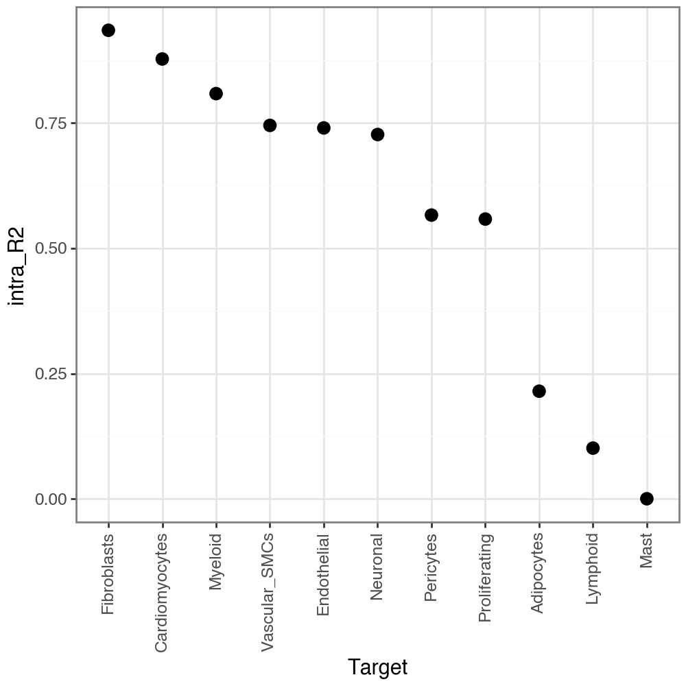
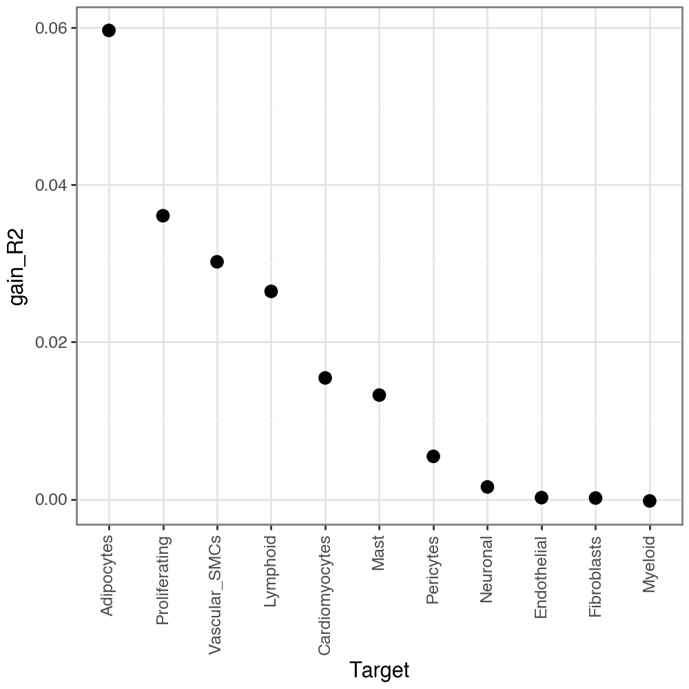
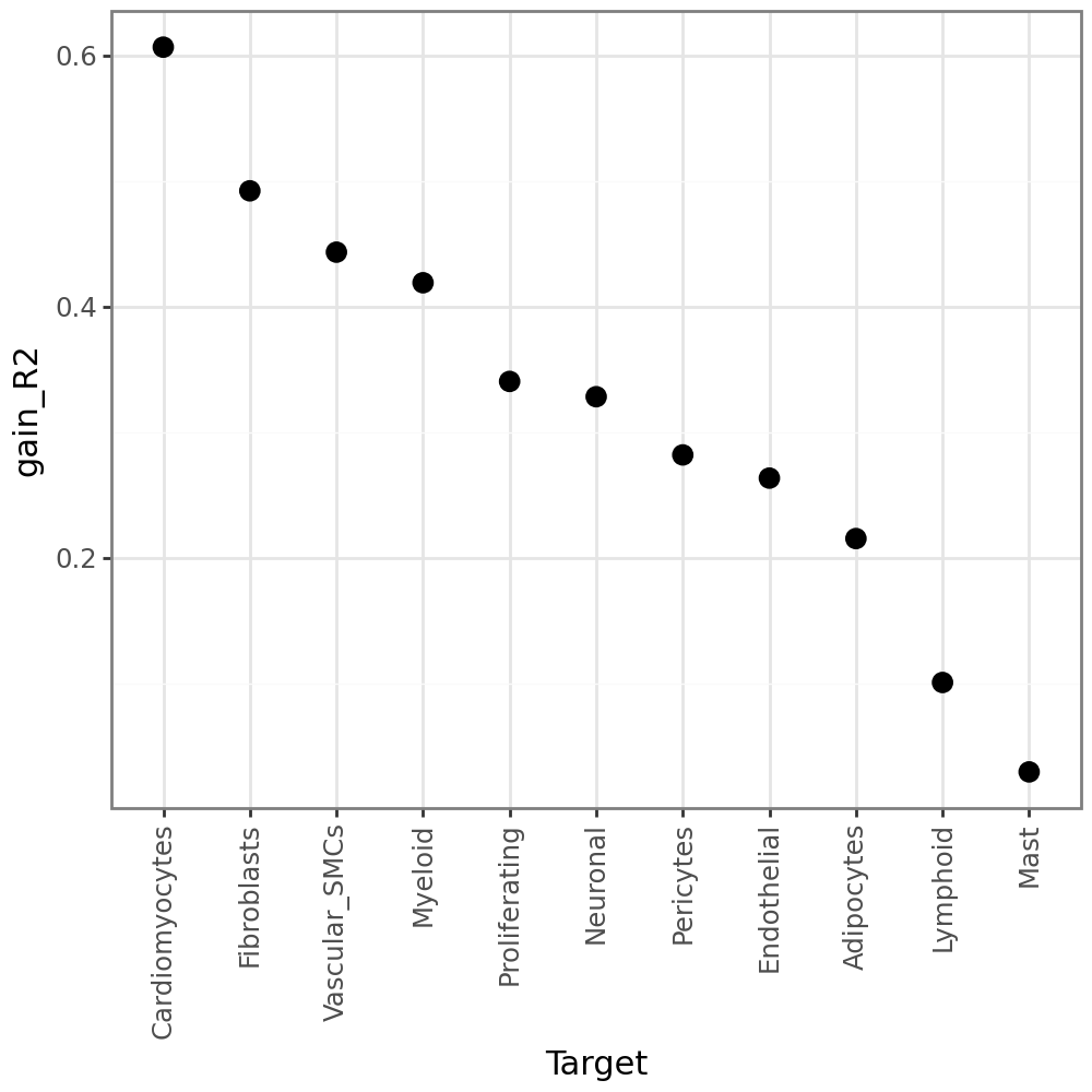
MISTy additionally calculate gain_R2, or in other words the performance gain when we additionally consider the other views (in addition to intra). When we look at the variance explained by the other views, we see that they explain a bit less (as expected), but still there is still some gain of predictive performance:

li.pl.target_metrics(misty, stat='gain_R2')

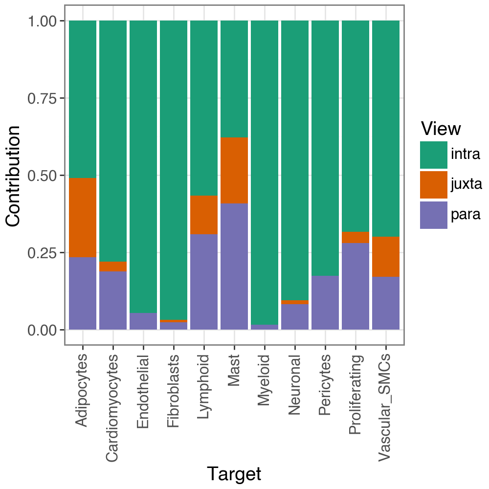
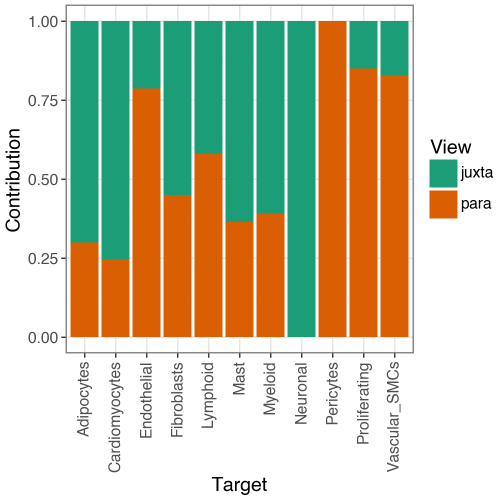
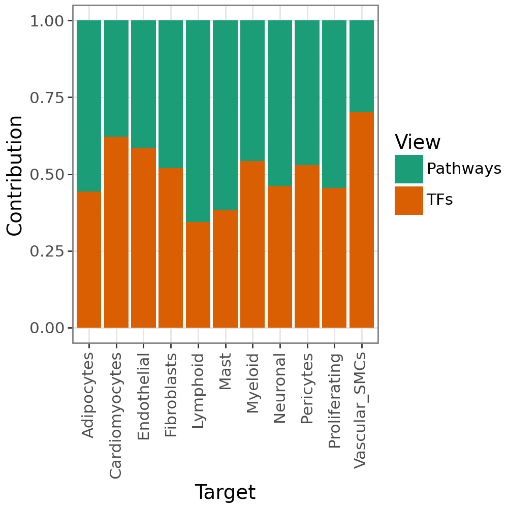
We can also check the contribution to the predictive performance of each view per target:

li.pl.contributions(misty, return_fig=True)

Finally, using the information above we know which variables are best explained by our model, and we know which view explains them best. So, we can now also see what are the specific variables that explain each target best:

# this information is stored here:
misty.uns['interactions'].head()

	target	predictor	view	importances
0	Adipocytes	Cardiomyocytes	intra	0.061007
1	Adipocytes	Endothelial	intra	0.073574
2	Adipocytes	Fibroblasts	intra	0.055111
3	Adipocytes	Lymphoid	intra	0.048662
4	Adipocytes	Mast	intra	0.147789

li.pl.interactions(misty, view='juxta', return_fig=True, figure_size=(7,5))

Linear Misty

We can also use a Linear model, while a bit more simplistic is much faster and more interpretable.

Moreover, we will bypass predicting the intraview with features within the intraview features (bypass_intra). This will allow us to see how well the other views explain the intraview, excluding the intraview itself.

misty(model=LinearModel, k_cv=10, seed=1337, bypass_intra=True, verbose = True)

Let’s check the joined R-squared for views:

li.pl.target_metrics(misty, stat='gain_R2', return_fig=True)

and their contributions per target:

li.pl.contributions(misty, return_fig=True)

Since this is a linear model, the coefficients would not be directly comparable (as are importances in a Random Forest). Thus, we use the coefficients’ t-values, as calculated by Ordinary Least Squares, which are signed and directly comparable.

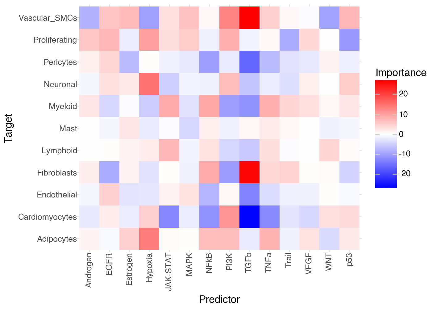
Let’s explore the t-values for each target-prediction interaction:

(
    li.pl.interactions(misty, view='juxta', return_fig=True, figure_size=(7,5)) + 
    p9.scale_fill_gradient2(low = "blue", mid = "white", high = "red", midpoint = 0)
)

Feature importances

Regardless of the model, each target is predicted independently, and the interpretation of feature importances depends on the model used. By default, we use a random forest, so the feature importances are the mean decrease in Gini impurity of the features. On the other hand, when we use a linear model, the feature importances are the t-values of the model coefficients.

Build Custom Misty Views

As we previously mentioned, one can build any view structure that they deem relevant for their data. So, let’s explore how to build custom views. Here, we will just use two distinct prior knowledge sources to check which one achieves better predictive performance.

So, let’s also estimate Transcription Factor activities with decoupler:

# get TF prior knowledge
net = dc.op.collectri(organism='human', remove_complexes=False, license='academic', verbose=False)

# Estimate activities
dc.mt.ulm(
    mat=adata,
    net=net,
    verbose=True,
    raw=False
)

---------------------------------------------------------------------------
TypeError                                 Traceback (most recent call last)
Cell In[30], line 2
      1 # Estimate activities
----> 2 dc.mt.ulm(
      3     mat=adata,
      4     net=net,
      5     verbose=True,
      6     raw=False
      7 )

TypeError: Method.__call__() missing 1 required positional argument: 'data'

# extract activities
acts_tfs = li.ut.obsm_to_adata(adata, 'score_ulm')

In addition to the features, we also need to provide spatial weights for the spots. Here, we will use LIANA’s inbuilt radial kernel function to compute spatial weights based on the spatial coordinates of the spots. However, this can be replaced by any other spatial weights matrix, such as those calculated via squidpy.gr.spatial_neighbors.

# Calculate spatial neighbors
li.ut.spatial_neighbors(acts_tfs, cutoff=0.1, bandwidth=200, set_diag=False)

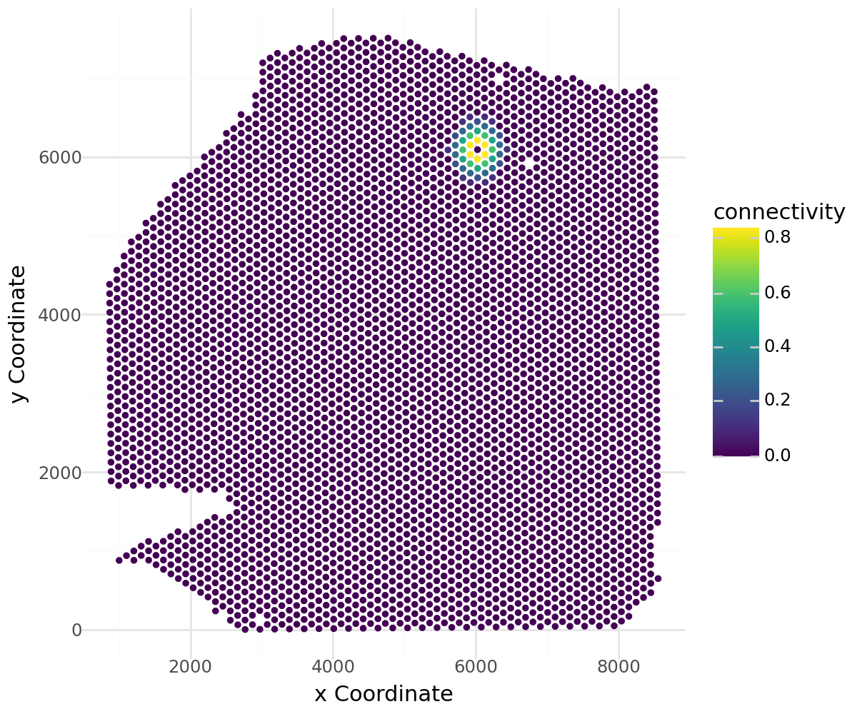
Visualize the weights for a specific spot:

li.pl.connectivity(acts_tfs, idx=0, figure_size=(6,5))

# transfer spatial information to progeny activities
# NOTE: spatial connectivities can differ between views, but in this case we will use the same
acts_progeny.obsm['spatial'] = acts_tfs.obsm['spatial']
acts_progeny.obsp['spatial_connectivities'] = acts_tfs.obsp['spatial_connectivities']

Build an object with custom views:

misty = MistyData(data={"intra": comps, "TFs": acts_tfs, "Pathways": acts_progeny})

misty

MuData object with n_obs × n_vars = 4113 × 719
  obs:	'in_tissue', 'array_row', 'array_col', 'sample', 'n_genes_by_counts', 'log1p_n_genes_by_counts', 'total_counts', 'log1p_total_counts', 'pct_counts_in_top_50_genes', 'pct_counts_in_top_100_genes', 'pct_counts_in_top_200_genes', 'pct_counts_in_top_500_genes', 'mt_frac', 'celltype_niche', 'molecular_niche'
  3 modalities
    intra:	4113 x 11
      obs:	'in_tissue', 'array_row', 'array_col', 'sample', 'n_genes_by_counts', 'log1p_n_genes_by_counts', 'total_counts', 'log1p_total_counts', 'pct_counts_in_top_50_genes', 'pct_counts_in_top_100_genes', 'pct_counts_in_top_200_genes', 'pct_counts_in_top_500_genes', 'mt_frac', 'celltype_niche', 'molecular_niche'
      uns:	'spatial', 'log1p', 'celltype_niche_colors'
      obsm:	'compositions', 'mt', 'spatial'
    TFs:	4113 x 694
      obs:	'in_tissue', 'array_row', 'array_col', 'sample', 'n_genes_by_counts', 'log1p_n_genes_by_counts', 'total_counts', 'log1p_total_counts', 'pct_counts_in_top_50_genes', 'pct_counts_in_top_100_genes', 'pct_counts_in_top_200_genes', 'pct_counts_in_top_500_genes', 'mt_frac', 'celltype_niche', 'molecular_niche'
      uns:	'spatial', 'log1p', 'celltype_niche_colors'
      obsm:	'compositions', 'mt', 'spatial', 'mlm_estimate', 'mlm_pvals', 'ulm_estimate', 'ulm_pvals'
      layers:	'weighted'
      obsp:	'spatial_connectivities'
    Pathways:	4113 x 14
      obs:	'in_tissue', 'array_row', 'array_col', 'sample', 'n_genes_by_counts', 'log1p_n_genes_by_counts', 'total_counts', 'log1p_total_counts', 'pct_counts_in_top_50_genes', 'pct_counts_in_top_100_genes', 'pct_counts_in_top_200_genes', 'pct_counts_in_top_500_genes', 'mt_frac', 'celltype_niche', 'molecular_niche'
      uns:	'spatial', 'log1p', 'celltype_niche_colors'
      obsm:	'compositions', 'mt', 'spatial', 'mlm_estimate', 'mlm_pvals'
      layers:	'weighted'
      obsp:	'spatial_connectivities'

Run Misty as before:

misty(model=LinearModel, verbose=True, bypass_intra=True)

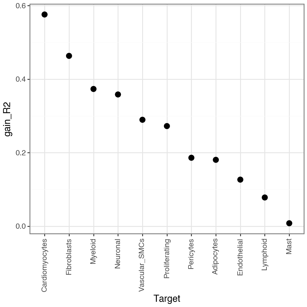
We can see that Cardiomyocytes and Fibroblasts are relatively well explained by TFs & Pathways.

li.pl.target_metrics(misty, stat='gain_R2')

We also see that the two views explain the targets similarly well.

li.pl.contributions(misty, return_fig=True)

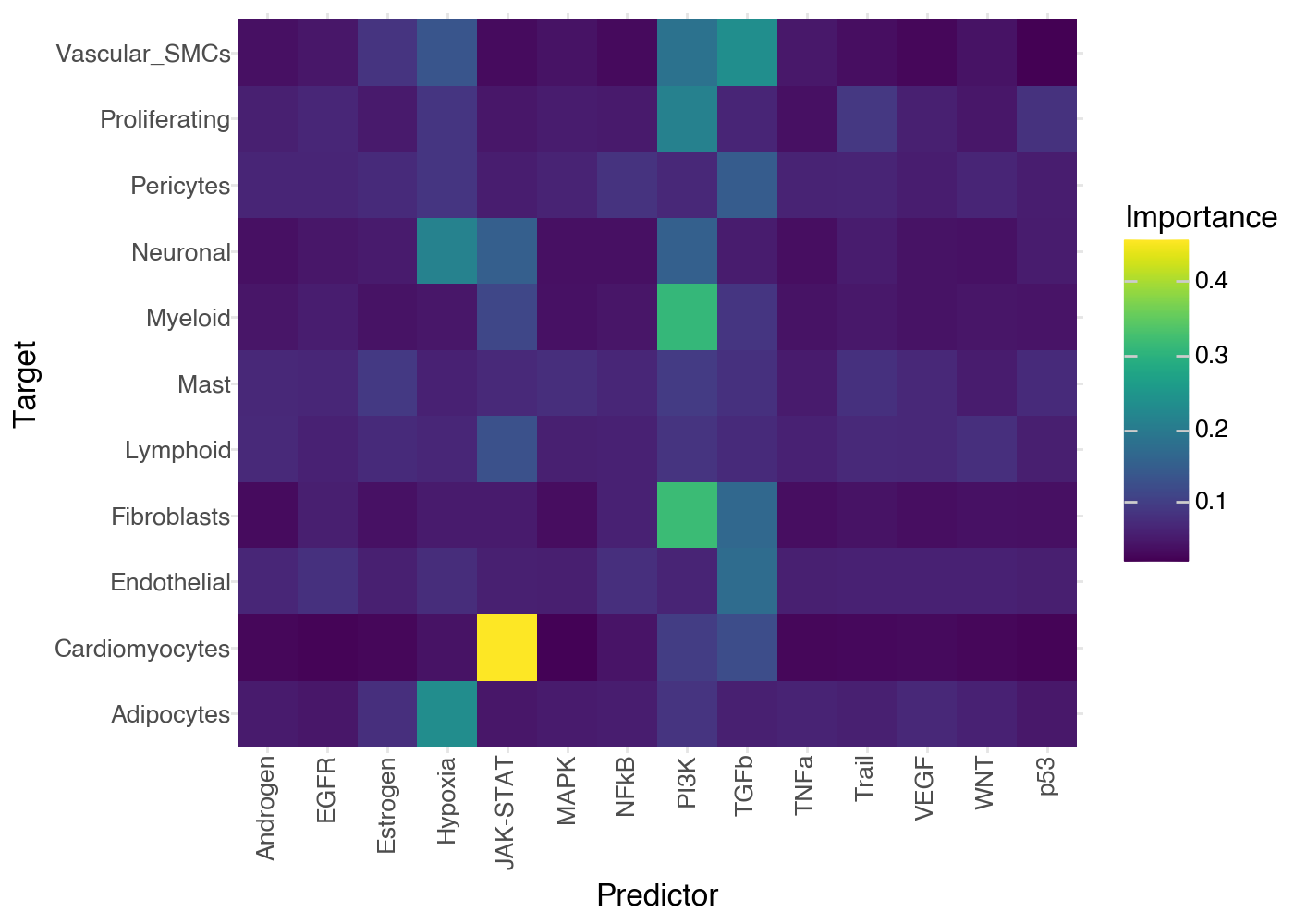
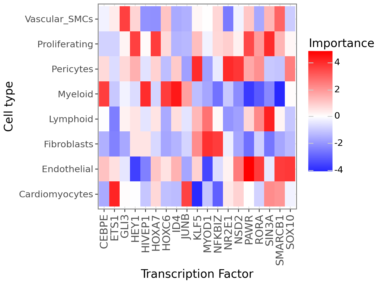
Plot cell type x Trascription factor interactions

(
    li.pl.interactions(misty, view='TFs', top_n=20) + 
    p9.labs(x='Transcription Factor', y='Cell type') +
    p9.theme_bw(base_size=14) +
    p9.theme(axis_text_x=p9.element_text(rotation=90, size=13)) +
    # change to blue-red
    p9.scale_fill_gradient2(low='blue', mid='white', high='red')
)

Ligand-Receptor Misty

Finally, we provide a utility function that builds an object with receptors in the intra view and ligands in the para view (or in their surrounding).

For the sake of computational speed, let’s identify the highly variable genes

sc.pp.highly_variable_genes(adata)
hvg = adata.var[adata.var['highly_variable']].index

Build LR Misty object:

misty = lrMistyData(adata[:, hvg], bandwidth=200, set_diag=False, cutoff=0.01, nz_threshold=0.1)

misty(bypass_intra=True, model=LinearModel, verbose=True)

Let’s now explore the top interactions between the ligands and receptors:

(
    li.pl.interactions(misty, view='extra', return_fig=True, figure_size=(6, 5), top_n=25, key=abs) + 
    p9.scale_fill_gradient2(low = "blue", mid = "white", high = "red", midpoint = 0) +
    p9.labs(y='Receptor', x='Ligand')
)

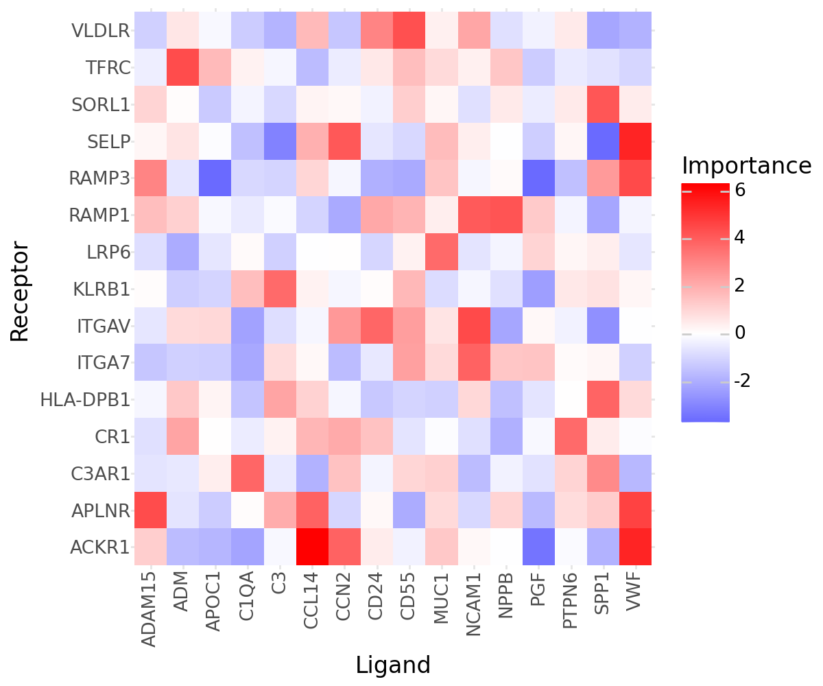
In contrast to any other other functions in LIANA, misty will infer all possible interactions between ligands and receptors - i.e. not only those that were annotated specifically as ligand-receptor interactions.

While this can be seen as a limitation, it can also be seen as an advantage of MISTy, as it allows us to explore potential ligand-receptor interactions that were not previously annotated!

While MISTy provides a flexible framework for the inference of spatially-informed interactions, it only summarizes relationships between the variables on the level of the whole slide (or niche); one should thus consider LIANA+'s bivariate local functions. These are simple spatially-informed spatially-informed metrics calculated at the spot-/cell-level. Thus, one can use them to visualize and explore the local distribution of interactions with spatial context.

Citing MISTy:

If you use MISTy via LIANA+, please cite MISTy’s original publication (Tanevski et al., 2022)