Spatially-informed Bivariate Metrics

This tutorial provides an overview of the local scores implemented in LIANA+. These scores are used to identify spatially co-expressed ligand-receptor pairs. However, there also applicable to other types of spatially-informed bivariate analyses.

It provides brief explanations of the mathematical formulations of the scores; these include adaptation of bivariate Moran’s R, Pearson correlation, Spearman correlation, weighted Jaccard similarity, and Cosine similarity. The tutorial also showcases interaction categories (masks) and significance testing.

Environement Setup

import pandas as pd
import scanpy as sc
import decoupler as dc
import liana as li

from mudata import MuData

Load and Normalize Data

To showcase LIANA’s local functions, we will use an ischemic 10X Visium spatial slide from Kuppe et al., 2022. It is a tissue sample obtained from a patient with myocardial infarction, focusing on the ischemic zone of the heart tissue.

The slide provides spatially-resolved information about the cellular composition and gene expression patterns within the tissue.

adata = sc.read("kuppe_heart19.h5ad", backup_url='https://figshare.com/ndownloader/files/41501073?private_link=4744950f8768d5c8f68c')
adata.layers['counts'] = adata.X.copy()
sc.pp.normalize_total(adata, target_sum=1e4)
sc.pp.log1p(adata)

adata.obs.head()

	in_tissue	array_row	array_col	sample	n_genes_by_counts	log1p_n_genes_by_counts	total_counts	log1p_total_counts	pct_counts_in_top_50_genes	pct_counts_in_top_100_genes	pct_counts_in_top_200_genes	pct_counts_in_top_500_genes	mt_frac	celltype_niche	molecular_niche
AAACAAGTATCTCCCA-1	1	50	102	Visium_19_CK297	3125	8.047510	7194.0	8.881142	24.770642	31.387267	39.797053	54.503753	0.085630	ctniche_1	molniche_9
AAACAATCTACTAGCA-1	1	3	43	Visium_19_CK297	3656	8.204398	10674.0	9.275660	35.956530	42.167885	49.456624	61.045531	0.033275	ctniche_5	molniche_3
AAACACCAATAACTGC-1	1	59	19	Visium_19_CK297	3013	8.011023	7339.0	8.901094	33.247036	39.910069	47.227143	59.326884	0.029139	ctniche_5	molniche_3
AAACAGAGCGACTCCT-1	1	14	94	Visium_19_CK297	4774	8.471149	14235.0	9.563529	22.739726	29.884089	37.850369	51.099403	0.149194	ctniche_7	molniche_2
AAACAGCTTTCAGAAG-1	1	43	9	Visium_19_CK297	2734	7.913887	6920.0	8.842316	35.664740	42.268786	50.000000	62.384393	0.025601	ctniche_5	molniche_3

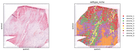
Spot clusters

sc.pl.spatial(adata, color=[None, 'celltype_niche'], size=1.3, palette='Set1')

Background

Here, we will demonstrate how to use the spatially-informed bivariate metrics to assess the spatial relationship between two variables. Specifically, we focus on local bivariate similarity metrics. In contrast to other spatial Methods, including Misty; focusing on local spatial relationships enables us to pinpoint the exact location of spatial relationships, and to identify spatial relationships that might occur only in a specific sub-region of our samples.

Following the initial concept of LIANA, and inspired by scHOT, we have natively re-implemented 6 local bivariate metrics, including scHOT’s (default) masked Spearman & SpatialDM’s local Moran’s R.

As part of the LIANA+ manuscript, we performed two distinct tasks to evaluate the ability of these metrics to preserve biological information, and saw that on average when used to identify local ligand-receptor relationships, spatially-weighted Cosine similarity did best. Thus, we will focus on it throughout this tutorial. However, we expect that other scoring functions might be better suited for other tasks, e.g. Spatially-weighted Jaccard Similarity should be well suited for categorical data; thus we encourage you to explore them.

Available Local Functions

li.mt.bivariate.show_functions()

	name	metadata	reference
0	pearson	weighted Pearson correlation coefficient	None
1	spearman	weighted Spearman correlation coefficient	None
2	cosine	weighted Cosine similarity	None
3	jaccard	weighted Jaccard similarity	None
4	product	simple weighted product	If vars are z-scaled = Lee's static (Lee 2021;...
5	norm_product	normalized weighted product	None
6	morans	Moran's R	Li, Z., Wang, T., Liu, P. and Huang, Y., 2022....
7	masked_spearman	masked & weighted Spearman correlation	Ghazanfar, S., Lin, Y., Su, X., Lin, D.M., Pat...

How do they work?

The local functions work are quite simple, as they are simply weighted versions of well-known similarity metrics. For example, the spatially-weighted version of Cosine similarity is defined as:

\[cosw_i(x,y) = \frac{\sum_{i=1}^n w_{ij} x_{i} y_{i}}{\sqrt{\sum_{i=1}^n w_{ij} x_{i}^2} \sqrt{\sum_{i=1}^n w_{ij} y_{i}^2}}\]

where for each spot i, we perform summation over all spots n, where w​ represents the spatial connectivity weights from spot i to every other spot j; for variables x and y.

Spatial Connectivity

The way that spatially-informed methods usually work is by making use of weights based on the proximity (or spatial connectivity) between spots/cells. These spatial connectivities are then used to calculate the metric of interest, e.g. Cosine similarity, in a spatially-informed manner.

The spatial weights in LIANA+ are by default defined as a family of radial kernels that use the inverse Euclidean distance between cells/spots to bind the weights between 0 and 1, with spots that are closest having the highest spatial connectivity to one another (1), while those that are thought to be too far to be in contact are assigned 0.

Key parameters of spatial_neighbors include: - bandwidth controls the radius of the spatial connectivities where higher values will result in a broader area being considered (controls the radius relative to the coordinates stored in adata.obsm['spatial']) - cutoff controls the minimum value that will be considered to have a spatial relationship (anything lower than the cutoff is set to 0). - kernel controls the distribution (shape) of the weights (‘gaussian’ by default) - set_diag sets the diagonal (i.e. the weight for each spot to itself) to 1 if True. NOTE: Here we set it to True as we expect many cells to be neighbors of themselves within a visium spot

As choosing an optimal bandwidith can be tricky, we provide the query_bandwidth function which uses a set of coordinates to provide an estimate of how many cell or spot neighbors are being considered for each spot over a range of bandwidths.

plot, _ = li.ut.query_bandwidth(coordinates=adata.obsm['spatial'], start=0, end=500, interval_n=20)
plot

<Figure Size: (640 x 480)>

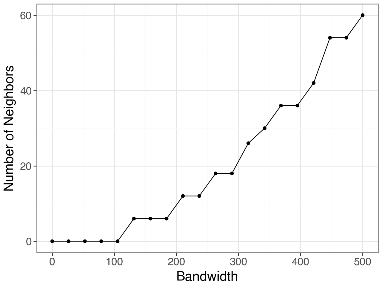
Here, we can see that a bandwidth of 150-200 (pixels) roughly includes 6 neighbours i.e. the first ring of neighbours in the hexagonal grid of 10x Visium. So, we will build the spatial graph with a bandwidth of 200.

li.ut.spatial_neighbors(adata, bandwidth=200, cutoff=0.1, kernel='gaussian', set_diag=True)

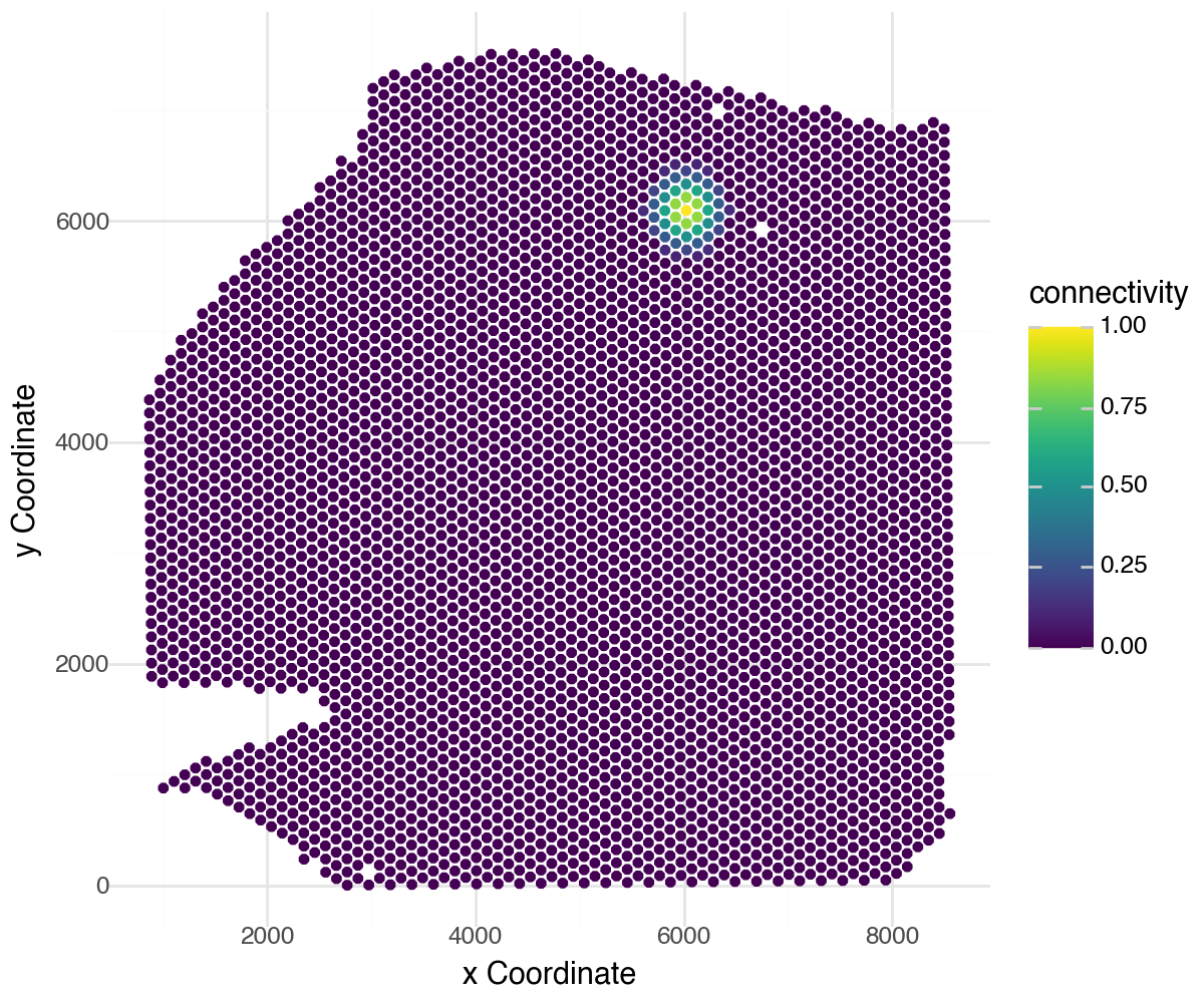
Let’s visualize the spatial weights for a single spot to all other spots in the dataset:

li.pl.connectivity(adata, idx=0, size=1.3, figure_size=(6, 5))

Fontsize 0.00 < 1.0 pt not allowed by FreeType. Setting fontsize = 1 pt

<Figure Size: (600 x 500)>

LIANA’s connectivities are flexible and can be defined in any way that fits the user. We have thus aligned LIANA’s spatial_neighbors function to Squidpy’s spatial_neighbors function. A perfectly viable solution would be to use Squidpy’s nearest neighbors graph, which one can use to easily replace LIANA’s radial kernel connecitivies.

Bivariate Ligand-Receptor Relationships

Now that we have covered the basics, let’s see how these scores look for potential ligand-receptor interactions on our 10X Visium Slide. Note that LIANA+ will take the presence of heteromeric complexes into account at the individual spot-level!

li.mt.bivariate(adata,
                resource_name='consensus', # Name of the LR resource
                local_name='cosine', # Name of the function
                global_name="morans", # Name global function
                n_perms=100, # Number of permutations to calculate a p-value
                mask_negatives=False, # Whether to mask LowLow/NegativeNegative interactions
                add_categories=True, # Whether to add local categories to the results
                nz_prop=0.2, # Minimum expr. proportion for ligands/receptors and their subunits
                use_raw=False,
                verbose=True
                )

Using `.X`!
Using resource `consensus`.
100%|██████████| 100/100 [01:56<00:00,  1.17s/it]
100%|██████████| 100/100 [01:01<00:00,  1.64it/s]

Now that this is done, we can extract and explore the newly-created AnnData object that counts our local scores

lrdata = adata.obsm['local_scores']

In addition to the local bivariate scores, we can also get the “global” scores for each pair of variables, which we can choose the best pairs of variables to visualize:

lrdata.var.sort_values("mean", ascending=False).head(3)

	ligand	receptor	ligand_means	ligand_props	receptor_means	receptor_props	morans	morans_pvals	mean	std
interaction
TIMP1^CD63	TIMP1	CD63	3.048890	0.996839	2.887192	0.994165	0.033729	0.0	0.981958	0.013757
LGALS1^ITGB1	LGALS1	ITGB1	3.534027	0.997326	2.457884	0.988330	0.149732	0.0	0.978951	0.027114
LUM^ITGB1	LUM	ITGB1	3.173511	0.996353	2.457884	0.988330	-0.103130	0.0	0.963635	0.026913

lrdata.var.sort_values("std", ascending=False).head(3)

	ligand	receptor	ligand_means	ligand_props	receptor_means	receptor_props	morans	morans_pvals	mean	std
interaction
S100A1^RYR2	S100A1	RYR2	0.697087	0.572332	0.430792	0.406516	0.271809	0.0	0.489952	0.259712
VTN^ITGAV_ITGB5	VTN	ITGAV_ITGB5	0.434514	0.395089	1.108789	0.814977	0.161359	0.0	0.545211	0.234249
LPL^VLDLR	LPL	VLDLR	0.791770	0.609531	0.612294	0.540725	0.220095	0.0	0.572516	0.231662

We can also use Global bivariate Moran’s R (or Lee’s statistic) - an extension of univariate Moran’s I, as proposed by Anselin 2019 and Lee and Li, 2019; implemented initially in [SEAGAL] SpatialDM.

A useful property of Bivariate Moran’s R is that it is bound between -1 (perfect negative spatial co-expression) and 1 (perfect positive spatial co-expression). Thus, it can be used to identify pairs of variables that are spatially clustered together, or apart.

lrdata.var.sort_values("morans", ascending=False).head()

	ligand	receptor	ligand_means	ligand_props	receptor_means	receptor_props	morans	morans_pvals	mean	std
interaction
APOE^LRP1	APOE	LRP1	1.179983	0.752006	1.937682	0.956236	0.284863	0.0	0.802385	0.142088
S100A1^RYR2	S100A1	RYR2	0.697087	0.572332	0.430792	0.406516	0.271809	0.0	0.489952	0.259712
SERPING1^LRP1	SERPING1	LRP1	1.711175	0.931437	1.937682	0.956236	0.243950	0.0	0.906663	0.077607
VTN^ITGAV_ITGB1	VTN	ITGAV_ITGB1	0.434514	0.395089	1.713479	0.929006	0.235151	0.0	0.592883	0.231178
MDK^LRP1	MDK	LRP1	1.127114	0.789691	1.937682	0.956236	0.227208	0.0	0.829393	0.118597

From these Global summaries, we see that the average Cosine similarity largely represents coverage - e.g. TIMP1 & CD63 is ubiquoutesly and uniformly distributed across the slide.

On the other hand, among most variable interactions and with with the highest global morans R is e.g. VTN&ITGAV_ITGB5. This interaction is thus more likely to represent biological relationships, with distinct spatial clustering patterns.

So, let’s visualize both:

sc.pl.spatial(lrdata, color=['VTN^ITGAV_ITGB5', 'TIMP1^CD63'], size=1.4, vmax=1, cmap='magma')

... storing 'ligand' as categorical
... storing 'receptor' as categorical

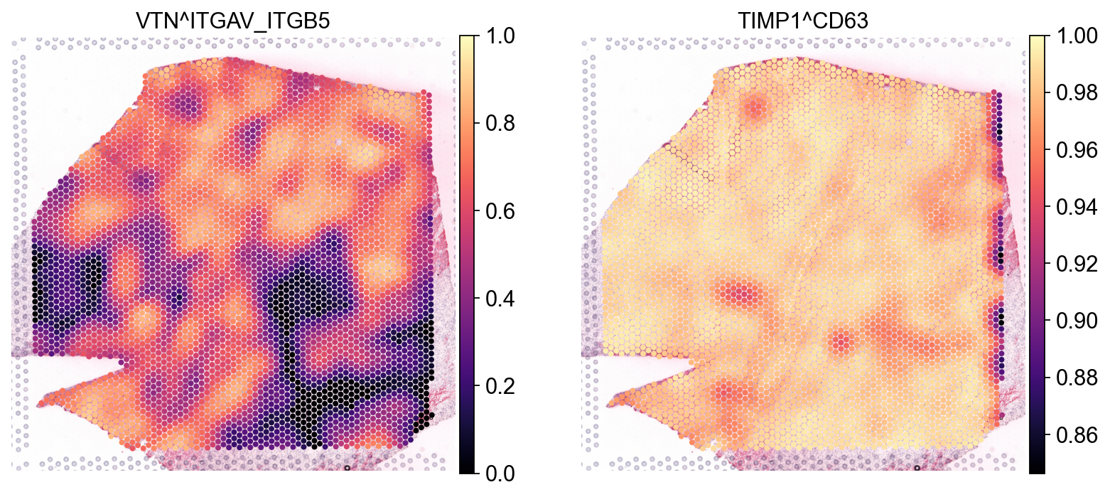
As expected, we see that the TIMP1 & CD63 interaction is uniformly distributed across the slide, while VTN&ITGAV_ITGB5 shows a clear spatial pattern.

We can also see that this is the case when we look at the individual genes:

sc.pl.spatial(adata, color=['VTN', 'ITGAV', 'ITGB5',
                            'TIMP1', 'CD63'],
              size=1.4, ncols=2)

While Moran’s R provides a sound summary of spatial clustering, it is limited to two variables at a time and is thus not fit for complex, or non-linear, spatial relationships between variables. Thus, we also encourage the user to explore LIANA+’s re-implementation of MISTy.

Permutation-based p-values

In addition to the local scores, we also calculated permutation-based p-values based on a null distribution generated by shuffling the spot labels. Let’s see how these look for the two interactions from above:

sc.pl.spatial(lrdata, layer='pvals', color=['VTN^ITGAV_ITGB5', 'TIMP1^CD63'], size=1.4, cmap="magma_r")

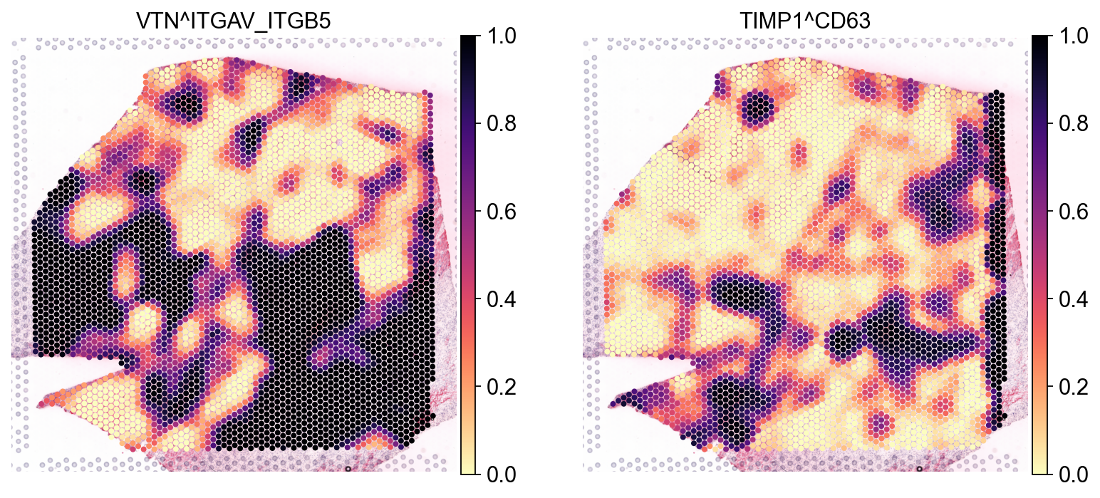
These largely agree with what we saw above for VTN&ITGAV_ITGB1 as appears to be specific to a certain region.

Local Categories

Did you notice that we used mask_negatives as a parameter when first estimating the interaction? This essentially means that we mask interactions in which both members are negative (or lowly expressed) when calculating the p-values, i.e. such which occur at places in which both members of the interaction are highly expressed. The locations at which both members are highly- expressed is defined as follows:

For each interaction, we define the category of both x and y for each spot as follows:

$$ Category_{i}(x) =

$$

Then we combine the categories of x and y for each spot, such that high-high are positive (1), high-low (or low-high) are -1; and low-low are 0. When working with non-negative values (i.e. gene expression); the features will be z-scaled (across observations).

sc.pl.spatial(lrdata, layer='cats', color=['VTN^ITGAV_ITGB5', 'TIMP1^CD63'], size=1.4, cmap="coolwarm")

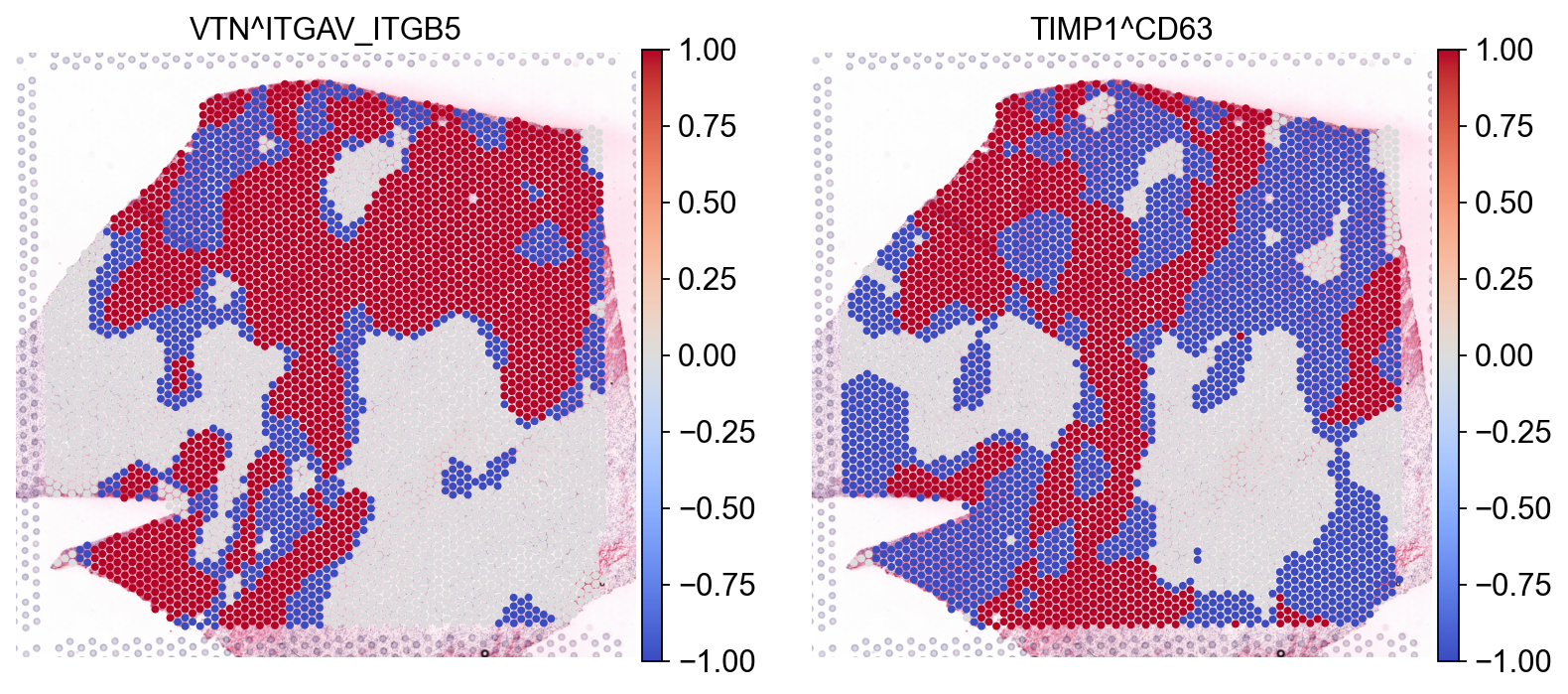
Here, we can distinguish areas in which the interaction between interaction members is positive (high-high) in Red (1), while interactions in which one is high the other is low or negative (High-low) are in Blue (-1). We also see that some interactions are neither, these are predominantly interactions in which both members are lowly-expressed (i.e. low-low); we see those in white (0).

When set to mask_negatives=False, we also return interactions that are not between necessarily positive/high magnitude genes ; when set to mask_negatives=True, we mask interactions that are negative (low-low) or uncategorized; for both the p-values and the local scores.

Identify Intercellular Patterns

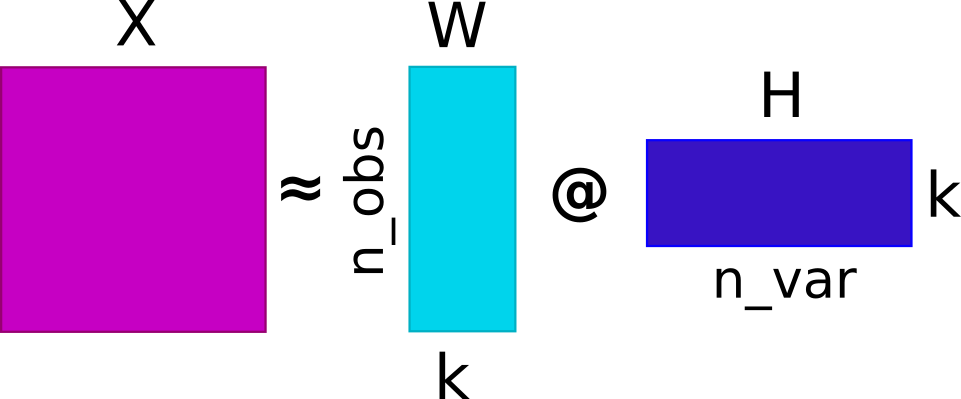
Now that we have estimated ligand-receptor scores, we can use non-negative matrix factorization (NMF) to identify coordinated cell-cell communication signatures. This would ultimately decompose the ligand-receptor scores into a basis matrix (W) and a coefficient matrix (H). We will use a very simple utility function (around sklearn’s NMF implementation) to do so, along with a simple k (component number) selection procedure.

• Basis Matrix (W): Each basis vector represents a characteristic pattern of ligand-receptor expression in the dataset. The values in W (factor score) indicate the strengths of factor in each spot; high values indicate high influence by the associated communication signature, while low values mean a weak influence.

• Coefficient Matrix (H): Each row of H represents the participation of the corresponding sample in the identified factor. The elements of each basis vector indicate the contribution of different interactions to the pattern (factor).

By decomposing the ligand-receptor interactions into W and H, NMF can potentially identify underlying CCC processes, with additive and non-negative relationships between the features. This property aligns well with the biological intuition that genes work together in a coordinated manner, but assumes linearity and only captures additive effects. Thus, alternative decomposition or clustering approaches can be used to a similar end.

In this particular scenario, we chose NMF as it is a well-established method for decomposition of non-negative matrices, it is fast, and it is easy to interpret. Also, in our case the ligand-receptor local scores already encode the spatial relationships between the features, so we don’t necessarily need to use a spatial-aware decomposition methods (e.g. SpatialDE, Spatial NMF, Chrysalis, or MEFISTO).

One limitation of NMF is that it requires the number of components (factors) to be specified - a somewhat an arbitrary choice. To aid the selection of n_components, we provide a simple function that estimates an elbow based on reconstruction error. Another limitation is that it only accepts non-negative values, so it won’t work with metrics that can be negative (e.g. Pearson correlation). In this case, we use Cosine similarity with non-negative values, which results also in non-negative local scores.

li.multi.nmf(lrdata, n_components=None, inplace=True, random_state=0, max_iter=200, verbose=True)

  0%|          | 0/10 [00:00<?, ?it/s]/home/dbdimitrov/anaconda3/envs/spiana/lib/python3.10/site-packages/sklearn/decomposition/_nmf.py:1710: ConvergenceWarning: Maximum number of iterations 200 reached. Increase it to improve convergence.
 10%|█         | 1/10 [00:02<00:25,  2.86s/it]/home/dbdimitrov/anaconda3/envs/spiana/lib/python3.10/site-packages/sklearn/decomposition/_nmf.py:1710: ConvergenceWarning: Maximum number of iterations 200 reached. Increase it to improve convergence.
 20%|██        | 2/10 [00:08<00:34,  4.33s/it]/home/dbdimitrov/anaconda3/envs/spiana/lib/python3.10/site-packages/sklearn/decomposition/_nmf.py:1710: ConvergenceWarning: Maximum number of iterations 200 reached. Increase it to improve convergence.
 30%|███       | 3/10 [00:14<00:36,  5.20s/it]/home/dbdimitrov/anaconda3/envs/spiana/lib/python3.10/site-packages/sklearn/decomposition/_nmf.py:1710: ConvergenceWarning: Maximum number of iterations 200 reached. Increase it to improve convergence.
 40%|████      | 4/10 [00:21<00:35,  5.91s/it]/home/dbdimitrov/anaconda3/envs/spiana/lib/python3.10/site-packages/sklearn/decomposition/_nmf.py:1710: ConvergenceWarning: Maximum number of iterations 200 reached. Increase it to improve convergence.
 50%|█████     | 5/10 [00:29<00:32,  6.56s/it]/home/dbdimitrov/anaconda3/envs/spiana/lib/python3.10/site-packages/sklearn/decomposition/_nmf.py:1710: ConvergenceWarning: Maximum number of iterations 200 reached. Increase it to improve convergence.
 60%|██████    | 6/10 [00:37<00:28,  7.21s/it]/home/dbdimitrov/anaconda3/envs/spiana/lib/python3.10/site-packages/sklearn/decomposition/_nmf.py:1710: ConvergenceWarning: Maximum number of iterations 200 reached. Increase it to improve convergence.
 70%|███████   | 7/10 [00:47<00:23,  7.94s/it]/home/dbdimitrov/anaconda3/envs/spiana/lib/python3.10/site-packages/sklearn/decomposition/_nmf.py:1710: ConvergenceWarning: Maximum number of iterations 200 reached. Increase it to improve convergence.
 80%|████████  | 8/10 [00:56<00:16,  8.35s/it]/home/dbdimitrov/anaconda3/envs/spiana/lib/python3.10/site-packages/sklearn/decomposition/_nmf.py:1710: ConvergenceWarning: Maximum number of iterations 200 reached. Increase it to improve convergence.
 90%|█████████ | 9/10 [01:06<00:08,  8.88s/it]/home/dbdimitrov/anaconda3/envs/spiana/lib/python3.10/site-packages/sklearn/decomposition/_nmf.py:1710: ConvergenceWarning: Maximum number of iterations 200 reached. Increase it to improve convergence.
100%|██████████| 10/10 [01:17<00:00,  7.79s/it]
Estimated rank: 3
/home/dbdimitrov/anaconda3/envs/spiana/lib/python3.10/site-packages/sklearn/decomposition/_nmf.py:1710: ConvergenceWarning: Maximum number of iterations 200 reached. Increase it to improve convergence.

# Extract the variable loadings
lr_loadings = li.ut.get_variable_loadings(lrdata, varm_key='NMF_H').set_index('index')

# Extract the factor scores
factor_scores = li.ut.get_factor_scores(lrdata, obsm_key='NMF_W')

Convert NMF Factor scores to an AnnData object for plotting

nmf = sc.AnnData(X=lrdata.obsm['NMF_W'],
                 obs=lrdata.obs,
                 var=pd.DataFrame(index=lr_loadings.columns),
                 uns=lrdata.uns,
                 obsm=lrdata.obsm)

sc.pl.spatial(nmf, color=[*nmf.var.index, None], size=1.4, ncols=2)

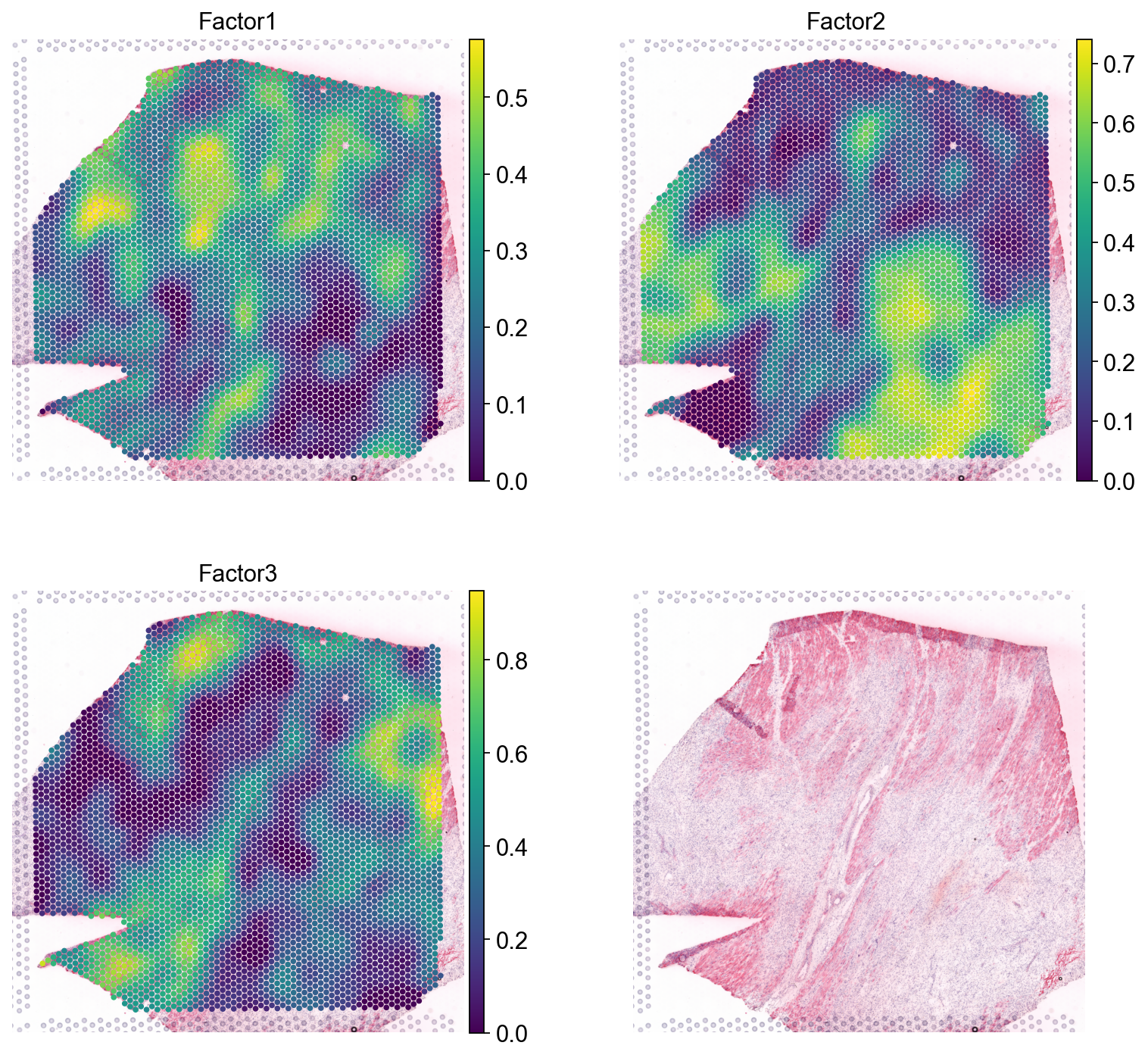
Wee see that Factor 2 is largely covering the ischemic areas of the side, let’s check the interactions contributing the most to it:

lr_loadings.sort_values("Factor2", ascending=False).head(10)

	Factor1	Factor2	Factor3
index
APOE^LRP1	1.301646	1.277514	0.314726
MDK^LRP1	1.424609	1.208298	0.373209
C3^LRP1	0.861049	1.197818	0.176564
SERPING1^LRP1	1.533601	1.184908	0.552800
VCAN^ITGB1	1.528520	1.164367	0.655848
C3^CD81	0.742810	1.164207	0.228812
C1QB^LRP1	1.506631	1.162397	0.559764
PSAP^LRP1	1.571949	1.156683	0.680581
FBN1^ITGB1	1.530816	1.147669	0.701900
S100A9^CD68	1.294533	1.146112	0.376383

From here on, one can estimate pathway activities or look for downstream effects of these interactions, plot the interactions, etc. These utility functions in liana are covered in other tutorials, but also applicable here.

Beyond Ligand-Receptors

While protein-mediated ligand-receptor interactions are interesting, cell-cell communication is not limited to those alone. Rather it is a complex process that involves a variety of different mechanisms such as signalling pathways, metabolite-mediated signalling, and distinct cell types.

So, if such diverse mechanisms are involved in cell-cell communication, why should we limit ourselves to ligand-receptor interactions? Let’s see how we can use LIANA+ to explore other types of cell-cell communication.

One simple approach would be to check relationships e.g. between transcription factors and cell type proportions.

Extract Cell type Composition

This slide comes with estimated cell type proportions using cell2location; See Kuppe et al., 2022. Let’s extract from .obsm them to an independent AnnData object.

# let's extract those
comps = li.ut.obsm_to_adata(adata, 'compositions')
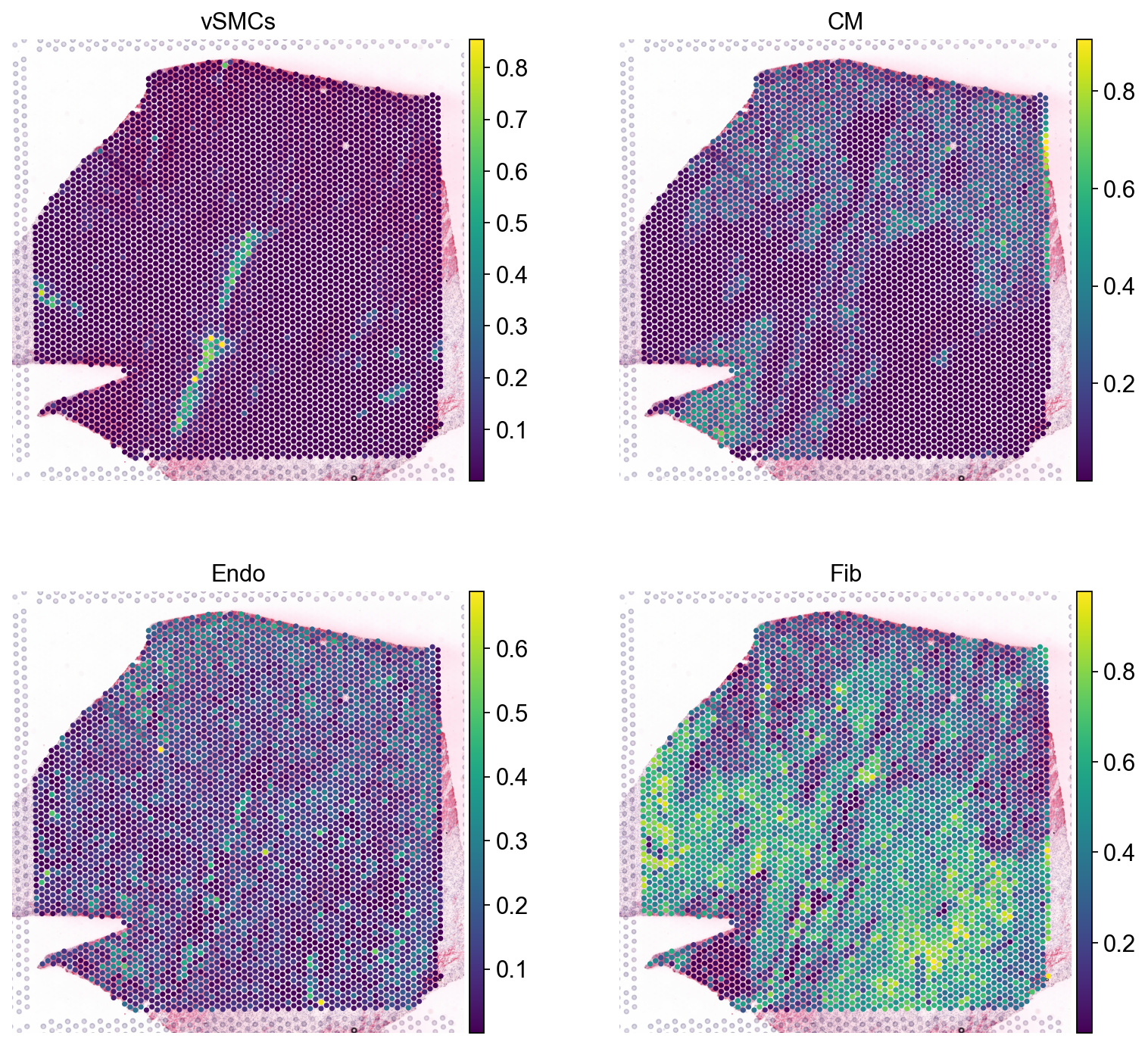
# check key cell types
sc.pl.spatial(comps, color=['vSMCs','CM', 'Endo', 'Fib'], size=1.3, ncols=2)

Estimate Transcription Factor Activity

# Get transcription factor resource
net = dc.get_collectri()

/home/dbdimitrov/anaconda3/envs/spiana/lib/python3.10/site-packages/tqdm/auto.py:21: TqdmWarning: IProgress not found. Please update jupyter and ipywidgets. See https://ipywidgets.readthedocs.io/en/stable/user_install.html
Downloading data from `https://omnipathdb.org/queries/enzsub?format=json`
Downloading data from `https://omnipathdb.org/queries/interactions?format=json`
Downloading data from `https://omnipathdb.org/queries/complexes?format=json`
Downloading data from `https://omnipathdb.org/queries/annotations?format=json`
Downloading data from `https://omnipathdb.org/queries/intercell?format=json`
Downloading data from `https://omnipathdb.org/about?format=text`

While multi-omics datasets might be even more of an interest, for the sake of simplicity (and because the general lack of spatial mutli-omics data at current times), let’s instead use enrichment analysis to estimate the activity of transcription factors in each spot. We will use one of decoupler-py’s enrichment methods with CollectTRI to do so. Refer to this tutorial for more info.

# run enrichment
dc.run_ulm(adata, net=net, use_raw=False, verbose=True)

Running ulm on mat with 4113 samples and 17703 targets for 694 sources.

100%|██████████| 1/1 [00:01<00:00,  1.36s/it]

Extract highly-variable TF activities

To reduce the number of TFs for the sake of computational speed, we will only focus on the top 50 most variable TFs.

Note we will use the simple coefficient of variation to identify the most variable TFs, but one can also use more sophisticated or spatially-informed methods to extract those (light-weight suggestions are welcome).

est = li.ut.obsm_to_adata(adata, 'ulm_estimate')
est.var['cv'] =  est.X.std(axis=0) / est.X.mean(axis=0)
top_tfs = est.var.sort_values('cv', ascending=False, key=abs).head(50).index

Create MuData object with TF activities and cell type proportions, and transfer spatial connectivities and other information from the original AnnData object.

mdata = MuData({"tf":est, "comps":comps})
mdata.obsp = adata.obsp
mdata.uns = adata.uns
mdata.obsm = adata.obsm

Define Interactions of interest:

from itertools import product

interactions = list(product(comps.var.index, top_tfs))

Estimate Cosine Similarity

li.mt.bivariate(mdata,
            x_mod="comps",
            y_mod="tf",
            x_transform=sc.pp.scale,
            y_transform=sc.pp.scale,
            local_name="cosine",
            interactions=interactions,
            mask_negatives=True,
            add_categories=True,
            x_use_raw=False,
            y_use_raw=False,
            xy_sep="<->",
            x_name='celltype',
            y_name='tf'
            )

To make the distributions comparable, we simply z-scale the TF activities and cell type proportions via the x_transform & y_transform parameters.

The type of transformation will affect the interpretation of the results, and different types of transformation might be more appropriate for different types of data. We provide zero-inflated minmax zi_minmax & neg_to_zero transformation functions via li.fun.transform.

One can explore how different transformations affect the results, to also get a better feeling how these local metrics work.

mdata.mod['local_scores'].var.sort_values("mean", ascending=False).head(5)

	celltype	tf	celltype_means	celltype_props	tf_means	tf_props	mean	std
interaction
CM<->TBX20	CM	TBX20	-4.452886e-09	1.0	-2.968591e-09	1.0	0.619449	0.161595
Fib<->SNAI2	Fib	SNAI2	-1.804437e-09	1.0	-1.382432e-09	1.0	0.563575	0.194297
Fib<->SOX6	Fib	SOX6	-1.804437e-09	1.0	1.461012e-08	1.0	0.505218	0.246272
Myeloid<->SNAI2	Myeloid	SNAI2	-4.758476e-09	1.0	-1.382432e-09	1.0	0.459984	0.220001
CM<->HAND1	CM	HAND1	-4.452886e-09	1.0	-1.059379e-08	1.0	0.456131	0.220627

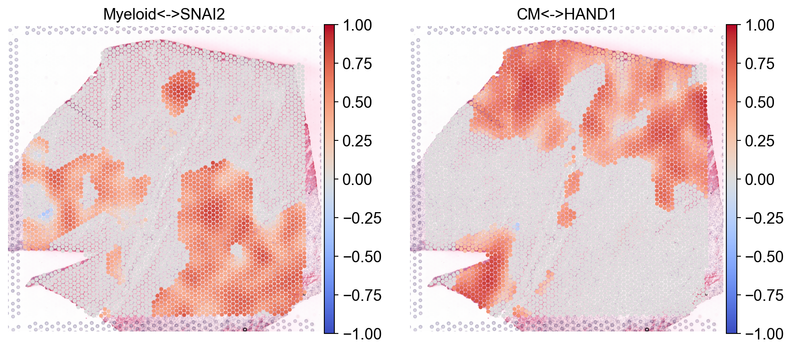
Let’s plot the results

sc.pl.spatial(mdata.mod['local_scores'], color=['Myeloid<->SNAI2', 'CM<->HAND1'], size=1.4, cmap="coolwarm", vmax=1, vmin=-1)

... storing 'celltype' as categorical
... storing 'tf' as categorical

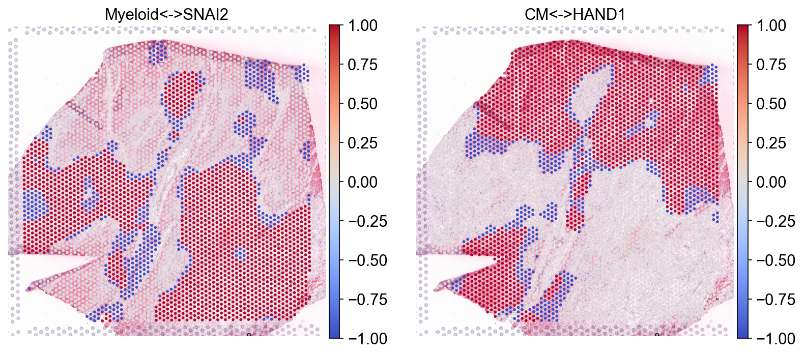
Plot categories

sc.pl.spatial(mdata.mod['local_scores'], layer='cats', color=['Myeloid<->SNAI2', 'CM<->HAND1'], cmap='coolwarm')

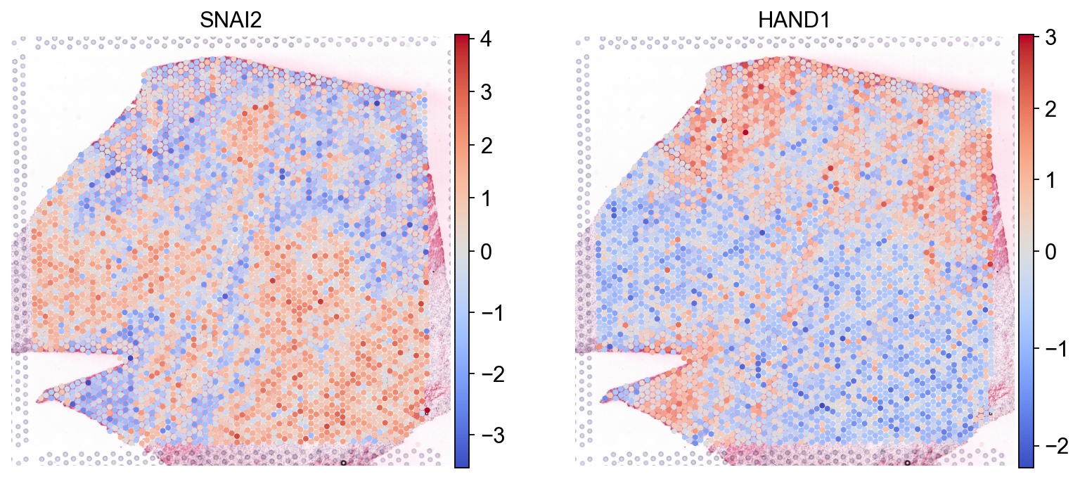
Plot variables (without transformations)

sc.pl.spatial(mdata.mod['tf'], color=['SNAI2', 'HAND1'], cmap='coolwarm', size=1.4, vcenter=0)

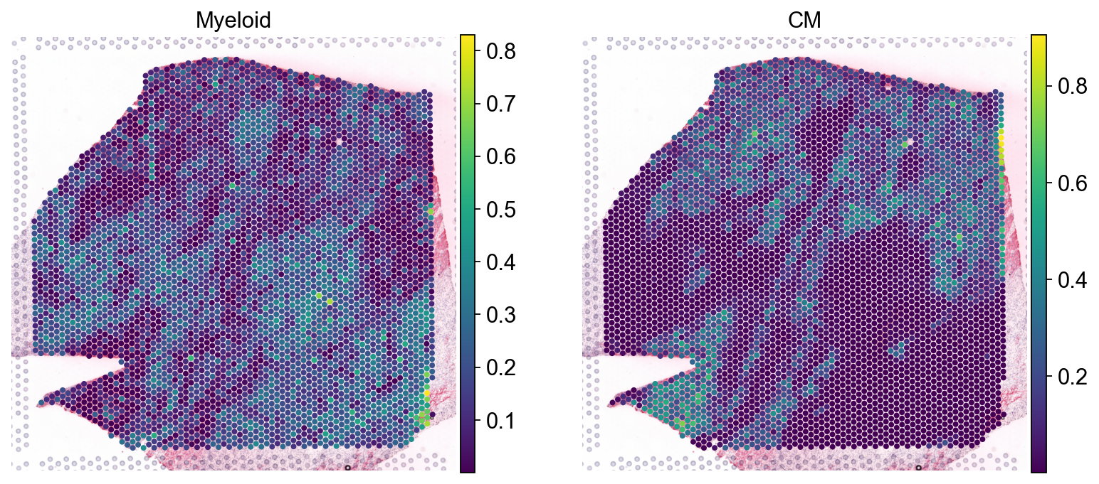
sc.pl.spatial(mdata.mod['comps'], color=['Myeloid', 'CM'], cmap='viridis', size=1.4)