Multi-Modal Ligand-Receptor Inference#
This notebook shows how to 1. analyse single-cell cite-seq data; 2. how to infer metabolite-receptor interactions from transcriptomics data.
import numpy as np
import pandas as pd
import scanpy as sc
import liana as li
import mudata as mu
from matplotlib import pyplot as plt
Infer Ligand-Receptor Interactions between RNA and Proteins#
Download Processed CITE-seq Data#
prot = sc.read('data/citeseq_prot.h5ad', backup_url='https://figshare.com/ndownloader/files/47625196')
rna = sc.read('data/citeseq_rna.h5ad', backup_url='https://figshare.com/ndownloader/files/47625193')
Load Processed CITE-Seq Data#
Here, we will use a very simple dataset to demonstrate the multi-modal ligand-receptor inference. We used a CITE-Seq dataset from 10X and followed the muon CITE-seq tutorial to process the RNA and Protein data.
Some minor differences are notable in the clustering due to the different versions of the packages used in the tutorial and the LIANA+ environment.
mdata = mu.MuData({'rna': rna, 'prot': prot})
# make sure that cell type is accessible
mdata.obs['celltype'] = mdata.mod['rna'].obs['celltype'].astype('category')
# inspect the object
mdata
MuData object with n_obs × n_vars = 3885 × 17838
  obs:	'celltype'
  var:	'gene_ids', 'feature_types', 'genome'
  2 modalities
    rna:	3885 x 17806
      obs:	'n_genes_by_counts', 'total_counts', 'total_counts_mt', 'pct_counts_mt', 'leiden', 'celltype'
      var:	'gene_ids', 'feature_types', 'genome', 'mt', 'n_cells_by_counts', 'mean_counts', 'pct_dropout_by_counts', 'total_counts', 'highly_variable', 'means', 'dispersions', 'dispersions_norm'
      uns:	'hvg', 'leiden', 'leiden_colors', 'log1p', 'neighbors', 'pca', 'rank_genes_groups', 'umap'
      obsm:	'X_pca', 'X_umap'
      obsp:	'connectivities', 'distances'
    prot:	3885 x 32
      var:	'gene_ids', 'feature_types', 'genome'
      uns:	'neighbors', 'pca', 'umap'
      obsm:	'X_pca', 'X_umap'
      varm:	'PCs'
      layers:	'counts'
      obsp:	'connectivities', 'distances'
Infer Interactions#
We see that we have two modalities, once for RNA and one for Proteins. We will next infer the ligand-receptor interactions between these two modalities.
CITE-seq data often focuses on antibody tagging of surface proteins, primarily receptors. To ensure only the protein modality is used for receptors, we append 'AB:' to receptor names in the antibody data. This step is necessary only when both RNA and antibody data have matching feature names.
# Obtain a ligand-receptor resource of interest
resource = li.rs.select_resource(resource_name='consensus')
# Append AB: to the receptor names
resource['receptor'] = 'AB:' + resource['receptor']

# Append AB: to the protein modality
mdata.mod['prot'].var_names = 'AB:' + mdata.mod['prot'].var['gene_ids']
While running LIANA+ with multimodal is largely analogous to when working with uni-modal data, there are a couple of things to keep in mind. Here, we need to ensure that the correct data is passed from each modality as well as to ensure that the correct modalities are used. Moreover, we need to ensure that data from the different modalities is comparable, which often requires the transformation of the data.
In this case, we use zero-inflated min-max normalization to ensure that the data from the two modalities is comparable. Essentially, a min-max normalization in which any value bellow 0.5 (by default) following normalization is set to 0. This normalization was originally introduced by the CiteFuse method, which is a ligand-receptor method for CITE-seq data.
li.mt.rank_aggregate(adata=mdata,
                     groupby='celltype',
                     # pass our modified resource
                     resource=resource,
                     # NOTE: Essential arguments when handling multimodal data
                     mdata_kwargs={
                     # Ligand-Receptor pairs are directed so we need to correctly pass
                     # `RNA` with ligands as `x_mod` and receptors as `y_mod`
                     'x_mod': 'rna',
                     'y_mod': 'prot',
                     # We use .X from the x_mod
                     'x_use_raw':False,
                     # We use .X from the y_mod
                     'y_use_raw':False,
                     # NOTE: we need to ensure that the modalities are correctly transformed
                     'x_transform':li.ut.zi_minmax,
                     'y_transform':li.ut.zi_minmax,
                    },
                  verbose=True
                  )
Using provided `resource`.
Transforming rna using zi_minmax
Transforming prot using zi_minmax
Generating ligand-receptor stats for 3885 samples and 37 features
Assuming that counts were `natural` log-normalized!
Running CellPhoneDB
Running Connectome
Running log2FC
Running NATMI
Running SingleCellSignalR
mdata.uns['liana_res'].head()
| source | target | ligand_complex | receptor_complex | lr_means | cellphone_pvals | expr_prod | scaled_weight | lr_logfc | spec_weight | lrscore | specificity_rank | magnitude_rank | |
|---|---|---|---|---|---|---|---|---|---|---|---|---|---|
| 1287 | pre-B | CD4+ memory T | HLA-DRA | AB:CD4 | 0.775442 | 0.0 | 0.600403 | 1.294984 | 0.643030 | 0.054068 | 0.968058 | 0.003006 | 0.000006 |
| 923 | mature B | CD4+ memory T | HLA-DRA | AB:CD4 | 0.772048 | 0.0 | 0.594934 | 1.284592 | 0.640910 | 0.053575 | 0.967917 | 0.003511 | 0.000022 |
| 1297 | pre-B | CD4+ naïve T | HLA-DRA | AB:CD4 | 0.756579 | 0.0 | 0.572285 | 1.246019 | 0.640179 | 0.051536 | 0.967308 | 0.003890 | 0.000050 |
| 936 | mature B | CD4+ naïve T | HLA-DRA | AB:CD4 | 0.753185 | 0.0 | 0.567072 | 1.235627 | 0.638059 | 0.051066 | 0.967163 | 0.003890 | 0.000089 |
| 1146 | pDC | CD4+ memory T | HLA-DRA | AB:CD4 | 0.751015 | 0.0 | 0.561047 | 1.220208 | 0.594210 | 0.050524 | 0.966993 | 0.003890 | 0.000138 |
Note that feature-wise min-max binds all features (i.e. genes and proteins) to the same limits, which essentially neglects the biological differences between features. This is typically not the case when working with untransformed data, as in that case we mostly care about cells being comparable, while features are typically with variable limits / distributions. As such, there might be some subtle differences from the interpretation of LIANA+ results, depending on the transformation of choice.
A benchmark of different normalizations for CCC are pending and alternative normalizations should also be explored. While other normalizations and subsequent transformations can also be used, the single-cell methods in LIANA+ require the data to be non-negative.
Plot Results & More#
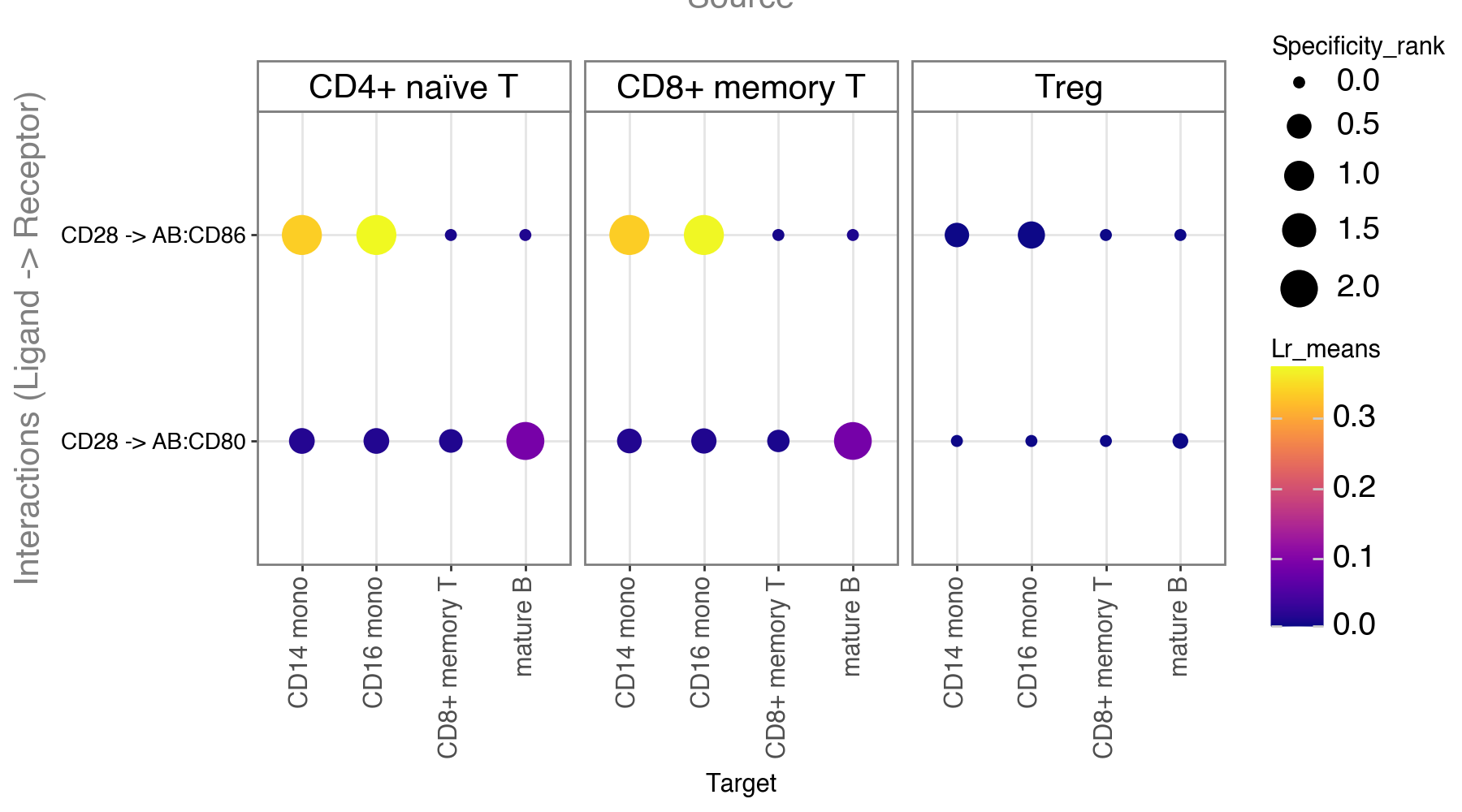
li.pl.dotplot(adata = mdata,
              colour='lr_means',
              size='specificity_rank',
              inverse_size=True, # we inverse sign since we want small p-values to have large sizes
              source_labels=['CD4+ naïve T', 'NK', 'Treg', 'CD8+ memory T'],
              target_labels=['CD14 mono', 'mature B', 'CD8+ memory T', 'CD16 mono'],
              figure_size=(9, 5),
              # finally, since cpdbv2 suggests using a filter to FPs
              # we filter the pvals column to <= 0.05
              filter_fun=lambda x: x['cellphone_pvals'] <= 0.05,
              cmap='plasma'
             )
Metabolite-mediated CCC from Transcriptomics Data#
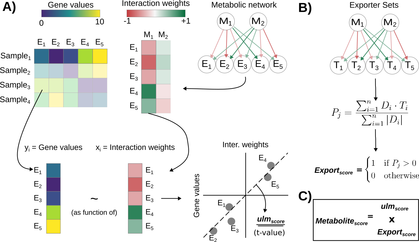
Recently, tools such as NeuronChat, MEBOCOST, scConnect, Cellinker, and CellPhoneDBv5 have proposed approaches, such as enrichment, expression average, among others, to infer metabolite-mediated CCC events from transcriptomics data. Similarly, we can use LIANA+ to infer metabolite-mediated CCC events from transcriptomics data, as described in the MetalinksDB manuscript.
Briefly, we use a univariate linear regression model to estimate metabolite abundances for each cell. To do so, we make use of production-degradation enzyme prior knowledge to infer the metabolite abundances. Optionally, we also take transporters into account. We then use these inferred metabolite abundances to infer metabolite-mediated CCC events.
Focus on Transcriptomics Data#
adata = mdata.mod['rna']
Obtain MetalinksDB Prior Knowledge#
Here, we will use MetalinksDB which contains prior knowledge about metabolite-receptor interactions as well as such for the production and degradation enzymes for metabolites. We will use the latter type of prior knowledge to infer the metabolite abundances for each cell.
metalinks = li.resource.get_metalinks(biospecimen_location='Blood',
                                      source=['CellPhoneDB', 'Cellinker', 'scConnect', # Ligand-Receptor resources
                                              'recon', 'hmr', 'rhea', 'hmdb' # Production-Degradation resources
                                              ],
                                      types=['pd', 'lr'], # NOTE: we obtain both ligand-receptor and production-degradation sets
                                     )
Prepare the Metabolite-Receptor Resource#
resource = metalinks[metalinks['type']=='lr'].copy()
resource = resource[['metabolite', 'gene_symbol']]\
    .rename(columns={'metabolite': 'source', 'gene_symbol': 'receptor'}).drop_duplicates()
resource.head()
| source | receptor | |
|---|---|---|
| 173 | Oxoglutaric acid | OXGR1 |
| 351 | Acetaldehyde | TRPA1 |
| 410 | Calcitriol | VDR |
| 843 | ADP | P2RY1 |
| 1071 | ADP | P2RY6 |
Prepare the Production-Degradation Network#
pd_net = metalinks[metalinks['type'] == 'pd']
# we need to aggregate the production-degradation values
pd_net = pd_net[['metabolite', 'gene_symbol', 'mor']].groupby(['metabolite', 'gene_symbol']).agg('mean').reset_index()
pd_net = pd_net.rename(columns={'metabolite': 'source', 'gene_symbol': 'target', 'mor': 'weight'})
pd_net.head()
| source | target | weight | |
|---|---|---|---|
| 0 | (+)-Limonene | CYP2C19 | -1.0 |
| 1 | (+)-Limonene | CYP2C9 | -1.0 |
| 2 | (R)-Lipoic acid | CEL | 1.0 |
| 3 | (R)-Lipoic acid | DLD | -1.0 |
| 4 | (R)-Lipoic acid | LIPA | 1.0 |
Prepare the transporter network#
t_net = metalinks[metalinks['type'] == 'pd']
t_net = t_net[['metabolite', 'gene_symbol', 'transport_direction']].dropna()
# Note that we treat export as positive and import as negative
t_net['mor'] = t_net['transport_direction'].apply(lambda x: 1 if x == 'out' else -1 if x == 'in' else None)
t_net = t_net[['metabolite', 'gene_symbol', 'mor']].dropna().groupby(['metabolite', 'gene_symbol']).agg('mean').reset_index()
t_net = t_net[t_net['mor']!=0]
t_net = t_net.rename(columns={'metabolite': 'source', 'gene_symbol': 'target', 'mor': 'weight'})
meta = li.mt.fun.estimate_metalinks(adata,
                                    resource,
                                    pd_net=pd_net,
                                    t_net=t_net,
                                    use_raw=False,
                                    tmin=3)
# pass cell type information
meta.obs['celltype'] = adata.obs['celltype']
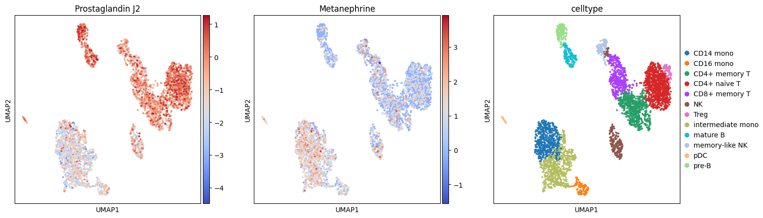
Essentially, we now have a dataset with two modalities, one for RNA and one for Metabolites. The metabolites are estimated as t-values. Let’s visualize a couple:
with plt.rc_context({"figure.figsize": (5, 5), "figure.dpi": (100)}):
    sc.pl.umap(meta.mod['metabolite'], color=['Prostaglandin J2', 'Metanephrine', 'celltype'], cmap='coolwarm')
Infer Metabolite-Receptor Interactions#
We will next infer the putative ligand-receptor interactions between these two modalities.
li.mt.rank_aggregate(adata=meta,
                     groupby='celltype',
                     # pass our modified resource
                     resource=resource.rename(columns={'source': 'ligand'}),
                     # NOTE: Essential arguments when handling multimodal data
                     mdata_kwargs={
                     'x_mod': 'metabolite',
                     'y_mod': 'receptor',
                     'x_use_raw':False,
                     'y_use_raw':False,
                     'x_transform':li.ut.zi_minmax,
                     'y_transform':li.ut.zi_minmax,
                    },
                  verbose=True
                  )
Using provided `resource`.
Transforming metabolite using zi_minmax
Transforming receptor using zi_minmax
Generating ligand-receptor stats for 3885 samples and 190 features
Assuming that counts were `natural` log-normalized!
Running CellPhoneDB
Running Connectome
Running log2FC
Running NATMI
Running SingleCellSignalR
Explore Results#
meta.uns['liana_res'].head()
| source | target | ligand_complex | receptor_complex | lr_means | cellphone_pvals | expr_prod | scaled_weight | lr_logfc | spec_weight | lrscore | specificity_rank | magnitude_rank | |
|---|---|---|---|---|---|---|---|---|---|---|---|---|---|
| 3446 | pre-B | NK | Prostaglandin J2 | PTGDR | 0.498391 | 0.0 | 0.170128 | 1.251590 | 0.361967 | 0.069165 | 0.736271 | 0.001834 | 7.902015e-07 |
| 2567 | mature B | NK | Prostaglandin J2 | PTGDR | 0.482969 | 0.0 | 0.163385 | 1.204872 | 0.341928 | 0.066424 | 0.732325 | 0.002293 | 3.160182e-06 |
| 1973 | Treg | NK | Prostaglandin J2 | PTGDR | 0.472941 | 0.0 | 0.159000 | 1.174493 | 0.321560 | 0.064641 | 0.729651 | 0.002528 | 7.109003e-06 |
| 1073 | CD4+ naïve T | NK | Prostaglandin J2 | PTGDR | 0.461330 | 0.0 | 0.153923 | 1.139322 | 0.345939 | 0.062577 | 0.726438 | 0.002999 | 1.263573e-05 |
| 781 | CD4+ memory T | NK | Prostaglandin J2 | PTGDR | 0.416395 | 0.0 | 0.134274 | 1.003198 | 0.259653 | 0.054589 | 0.712661 | 0.003013 | 5.050295e-05 |
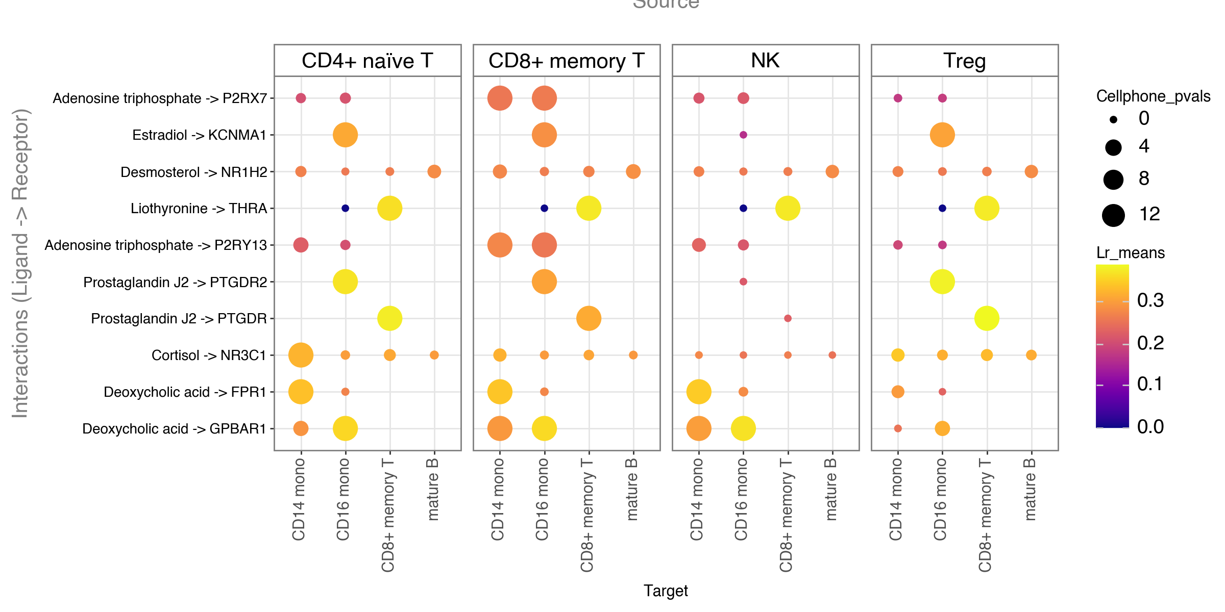
li.pl.dotplot(adata = meta,
              colour='lr_means',
              size='cellphone_pvals',
              inverse_size=True, # we inverse sign since we want small p-values to have large sizes
              source_labels=['CD4+ naïve T', 'NK', 'Treg', 'CD8+ memory T'],
              target_labels=['CD14 mono', 'mature B', 'CD8+ memory T', 'CD16 mono'],
              figure_size=(12, 6),
              # Filter to top 10 acc to magnitude rank
              top_n=10,
              orderby='magnitude_rank',
              orderby_ascending=True,
              cmap='plasma'
             )
Next Steps#
From here on one may follow-up with any of the other LIANA+ functionalities, such as plotting the results, or cross-conditional analyses.