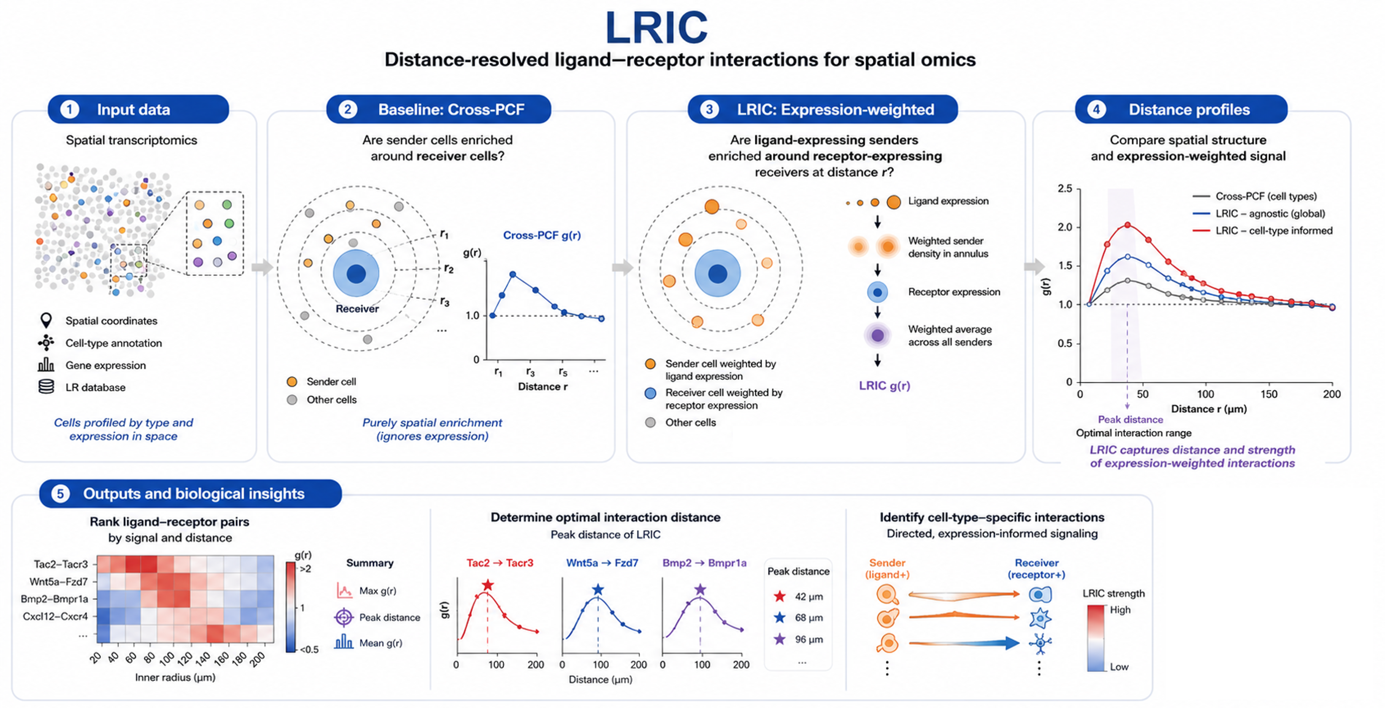
Ligand-Receptor Interaction Correlation (LRIC)

In this tutorial, we introduce LRIC, a weighted second-order spatial statistic in which pairwise contributions are weighted by ligand and receptor expression levels across a range of distances (annuli).

LRIC builds on the cross pair-correlation function (cross-PCF; see also Baddeley et al., 2016 and Bull et al., 2024) by additionally weighting every cell by its ligand and receptor expression.

Environement Setup

import os
import numpy as np
import pandas as pd
import matplotlib.pyplot as plt
import matplotlib.colors as mcolors
import scanpy as sc
import liana as li

Load and Normalize Data

To demonstrate the LRIC in practice, we will apply it to a spatial transcriptomics dataset from A molecularly defined and spatially resolved cell atlas of the whole mouse brain(Nature, 2023); WB_MERFISH_animal2_coronal.

The dataset was generated using MERFISH technique, which enables highly multiplexed single-molecule RNA imaging with subcellular spatial resolution. This dataset profiles the expression of more than 1,000 genes across roughly 10 million cells in the adult mouse brain.

file_path  = "data/MERFISH_mouse_brain/WB_MERFISH_animal2_coronal.h5ad"
backup_url = "https://datasets.cellxgene.cziscience.com/93c3bb97-ea05-4ee0-a760-a1508cd04612.h5ad"

adata = sc.read(file_path) if os.path.exists(file_path) else sc.read(file_path, backup_url=backup_url)

# Subset to one brain section
adata = adata[adata.obs["brain_section_label"] == "C57BL6J-2.039"]
# The dataset indexes vars by Ensembl ID; switch to gene symbols for LR lookup
adata.var_names = adata.var["gene_name"]

# Basic QC
sc.pp.filter_cells(adata, min_genes=10)
sc.pp.filter_genes(adata, min_cells=3)

# Normalise (keep raw counts in a layer); LRIC will use normalised log1p values
adata.layers["counts"] = adata.X.copy()
sc.pp.normalize_total(adata, target_sum=1e4)
sc.pp.log1p(adata)

# Spatial coordinates are in µm (MERFISH physical units)
print(adata)

AnnData object with n_obs × n_vars = 51539 × 1120
    obs: 'donor_id', 'development_stage_ontology_term_id', 'sex_ontology_term_id', 'self_reported_ethnicity_ontology_term_id', 'disease_ontology_term_id', 'tissue_ontology_term_id', 'cell_type_ontology_term_id', 'assay_ontology_term_id', 'suspension_type', 'cluster_id_transfer', 'subclass_transfer', 'cluster_confidence_score', 'subclass_confidence_score', 'high_quality_transfer', 'major_brain_region', 'ccf_region_name', 'brain_section_label', 'tissue_type', 'is_primary_data', 'cell_type', 'assay', 'disease', 'sex', 'tissue', 'self_reported_ethnicity', 'development_stage', 'observation_joinid', 'n_genes'
    var: 'gene_name', 'feature_is_filtered', 'feature_name', 'feature_reference', 'feature_biotype', 'feature_length', 'feature_type', 'n_cells'
    uns: 'citation', 'organism', 'organism_ontology_term_id', 'schema_reference', 'schema_version', 'title', 'log1p'
    obsm: 'X_CCF', 'X_spatial_coords', 'X_umap'
    layers: 'counts'

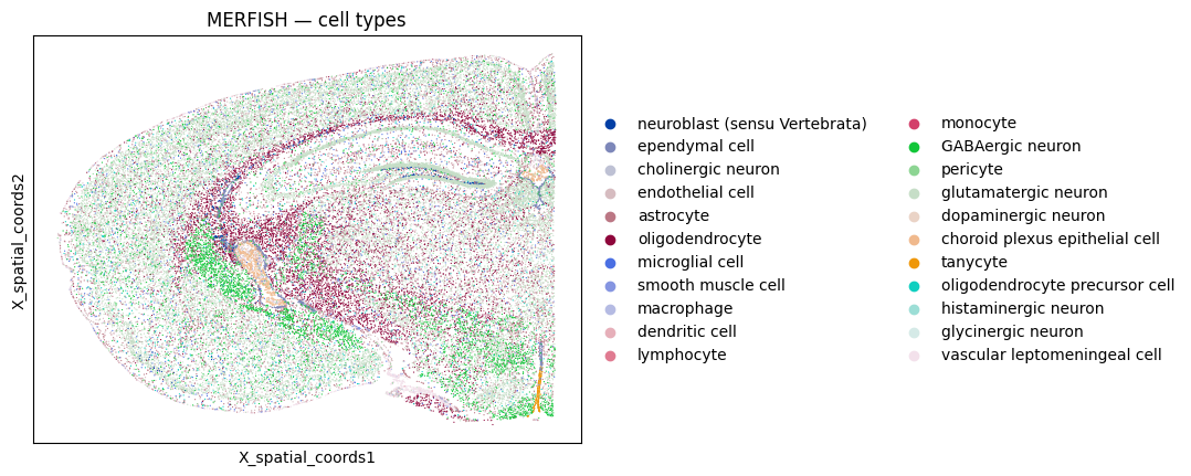
sc.pl.embedding(
    adata, basis="X_spatial_coords",
    color="cell_type", s=3, title="MERFISH — cell types"
)

Ligand–Receptor Database (mouse)

resource = li.rs.select_resource('mouseconsensus')
print(f"{len(resource)} LR pairs in resource")
resource.head(5)

3989 LR pairs in resource

	ligand	receptor
31371	Dll1	Notch1
31372	Dll1	Notch2
31373	Dll1	Notch4
31374	Dll1	Notch3
31375	Nrg2	Erbb2_Erbb3

Cross-PCF: Baseline Spatial Structure

Cross-PCF answers a purely spatial question:

Are cells of type B more (or less) frequent around cells of type A at distance r than expected under complete spatial randomness?

It treats all cells equally. Gene expression is not considered. We use it to characterise the raw spatial architecture of the tissue before asking about LR interactions.

The Cross-PCF adaptation implemented in LIANA+ was inspired by (Bull et al., 2024).

Choose the right parameters

All distance parameters are in the same units as the spatial coordinates µm for this MERFISH dataset.
radius_step = step between bin inner edges (e.g. 20-25 µm, the typical upper bound of the diameter of generic cells; though this might vary a lot depending on the tissue and cell types!).
annulus_width = radial width of each annulus ring.
Setting annulus_width = radius_step ensures bins are non-overlapping and tile the full range without gaps.
max_radius = inner edge of the last (widest) bin; the outer edge extends to max_radius + annulus_width.

annulus_width = 25

li.pl.annulus_plot(
    adata,
    spatial_key="X_spatial_coords",
    annulus_width=annulus_width,
    radius_step=annulus_width,
    n_rings=9,
    seed=5,
    figure_size= (6, 6))

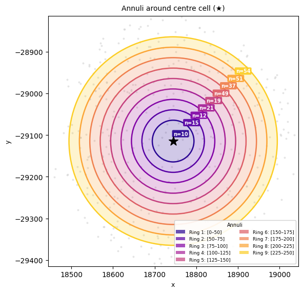
Note that, by default (extend_first_annulus=True), the innermost [0, radius_step) contact band is merged into the first annulus, which therefore spans [0, radius_step + annulus_width) and starts at radius 0. Distances are measured from each focal cell’s centroid, so cell centroids cannot lie closer than ~one cell diameter; the innermost band is otherwise a thin, near-empty, high-variance bin. Merging it folds genuine cell–cell contact pairs into the first bin instead of discarding them. Set extend_first_annulus=False to keep the first ring at [radius_step, radius_step + annulus_width).

Cross-PCF

li.mt.cross_pcf(
    adata,
    groupby="cell_type",
    spatial_key="X_spatial_coords",
    max_radius=200,
    radius_step=annulus_width,
    annulus_width=annulus_width,
    min_cells=50,
    key_added="cross_pcf", #results will be saved under this label in adata.uns
    verbose=True,
)

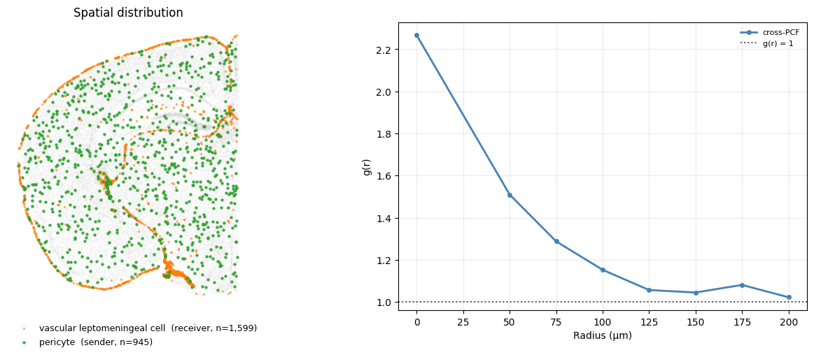
Aggregation: cells cluster together at a short distance

We will find cross-pcf results for Pericytes and vascular leptomeningeal cells (VLMCs), both are vascular support cell types associated with the perivascular niche and are expected to show spatial co-localisation along blood vessels.

cpcf = adata.uns["cross_pcf"]
r = np.asarray(cpcf["radii"], dtype=float)

snd, rcv = "pericyte", "vascular leptomeningeal cell"
crosspcf = np.asarray(cpcf["results"][(snd, rcv)], dtype=float)

We reuse the same two-panel summary throughout this section, so we wrap it in a small helper. plot_pair draws the spatial layout of a sender→receiver pair on the left and overlays their g(r) curve(s) on the right; optionally passing ligand/receptor annotates the legend with the fraction of each population expressing them.

def plot_pair(snd, rcv, curves, colors=None, title=None,
              ligand=None, receptor=None, spatial_key="X_spatial_coords"):
    """Two-panel summary for a sender -> receiver cell-type pair.

    Left: spatial map of the sender (green) and receiver (orange) cells over
    the rest of the tissue (grey). Right: the supplied g(r) curve(s) drawn with
    ``li.pl.lric_lineplot`` — ``curves`` maps each label to an ``(radii, g)``
    tuple. If ``ligand``/``receptor`` are given, the legend also reports the
    percentage of each population expressing them.
    """
    coords = adata.obsm[spatial_key]
    ct = adata.obs["cell_type"].astype(str).values
    snd_mask, rcv_mask = ct == snd, ct == rcv
    other_mask = ~(snd_mask | rcv_mask)

    snd_lab = f"{snd}  (sender, n={snd_mask.sum():,})"
    rcv_lab = f"{rcv}  (receiver, n={rcv_mask.sum():,})"
    if ligand is not None and receptor is not None:
        snd_pct = 100 * (adata[:, ligand].X.toarray()[snd_mask] > 0).mean()
        rcv_pct = 100 * (adata[:, receptor].X.toarray()[rcv_mask] > 0).mean()
        snd_lab = f"{snd}  (n={snd_mask.sum():,},  {ligand}+ {snd_pct:.1f}%)"
        rcv_lab = f"{rcv}  (n={rcv_mask.sum():,},  {receptor}+ {rcv_pct:.1f}%)"

    fig, axes = plt.subplots(1, 2, figsize=(13, 5), layout="constrained",
                             gridspec_kw={"width_ratios": [1.1, 1.0]})
    ax0 = axes[0]
    ax0.scatter(coords[other_mask, 0], coords[other_mask, 1],
                s=2, c="lightgray", alpha=0.1, linewidths=0, rasterized=True)
    # receiver first, sender on top so the sender layer is not buried
    ax0.scatter(coords[rcv_mask, 0], coords[rcv_mask, 1],
                s=6, c="tab:orange", alpha=0.6, linewidths=0, rasterized=True, label=rcv_lab)
    ax0.scatter(coords[snd_mask, 0], coords[snd_mask, 1],
                s=10, c="tab:green", alpha=0.9, linewidths=0, rasterized=True, label=snd_lab)
    ax0.set_aspect("equal"); ax0.axis("off")
    ax0.set_title("Spatial distribution")
    ax0.legend(frameon=False, fontsize=9, loc="upper left",
               bbox_to_anchor=(0, -0.02), ncol=1)

    li.pl.lric_lineplot(None, curves, overlay=True, colors=colors, title=title, ax=axes[1])
    plt.show()

plot_pair(snd, rcv, {"cross-PCF": (r, crosspcf)}, colors="steelblue")

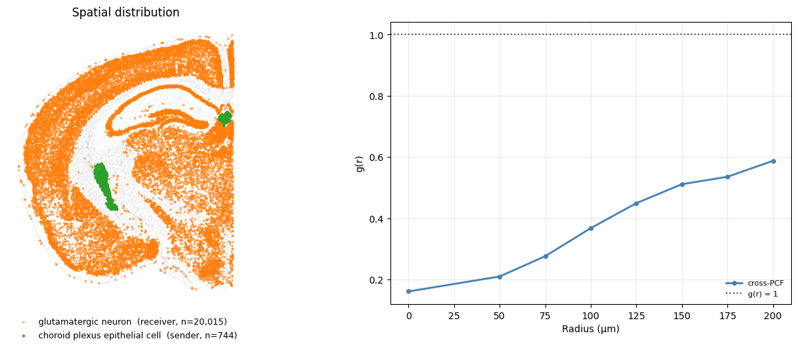
Exclusion: cells avoid each other

Choroid plexus epithelial cells are largely confined to the ventricular choroid plexus, while glutamatergic neurons are distributed throughout the brain parenchyma. Because these cell types occupy largely non-overlapping spatial domains, the observed cross-pair correlation function g(r) < 1 primarily reflects spatial compartmentalization.

snd, rcv = "choroid plexus epithelial cell", "glutamatergic neuron"
crosspcf = np.asarray(cpcf["results"][(snd, rcv)], dtype=float)

plot_pair(snd, rcv, {"cross-PCF": (r, crosspcf)}, colors="steelblue")

Ligand–Receptor Global Co-expression using LRIC

The agnostic mode of LRIC answer questions like:

Across all cells in the tissue, is the ligand signal spatially enriched around receptor-expressing receiver cells at distance r?

Here, because all cells are pooled, the signal can be inflated by tissue compartment structure, so a high agnostic score does not guarantee that the interaction is biologically directed between specific cell types.

li.mt.lric(
    adata,
    resource=resource,
    spatial_key="X_spatial_coords",
    max_radius=200,
    radius_step=annulus_width,
    annulus_width=annulus_width,
    use_raw=False,          
    key_added="lric_ag",  #results will be saved under this label in adata.uns
    verbose=True,
)

Using provided `resource`.

Rank LR Pairs by Signal

Useful summary statistics here:

• mean_lric: average g(r) across all radii (overall spatial co-enrichment).

• max_lric: peak g(r) (strength of the strongest spatial enrichment at any distance).

• peak_radius: distance at which g(r) is highest (characteristic interaction range).

ag = adata.uns["lric_ag"]
L = ag["lric"]

pair_scores = (
    pd.DataFrame({
        "pair": ag["pair_names"],
        "mean_lric": L.mean(0),
        "max_lric": L.max(0),
        "peak_radius": ag["radii"][L.argmax(0)],
    })
    .assign(max_minus_mean=lambda d: d["max_lric"] - d["mean_lric"])
    .sort_values("max_minus_mean", ascending=False)
)

top5 = pair_scores.head(5)

print("Top 5 LR pairs by (max - mean) LRIC:")
print(top5)

Top 5 LR pairs by (max - mean) LRIC:
               pair  mean_lric  max_lric  peak_radius  max_minus_mean
63       Ntf3^Ntrk3   2.456533  3.968962          0.0        1.512429
11      Col6a5^Cd44   1.848814  2.937120          0.0        1.088306
107  Gpc3^Tnfrsf11b   1.868091  2.910218          0.0        1.042127
95       Sfrp1^Fzd2   2.213429  3.238567          0.0        1.025138
92       Tac2^Tacr1   6.347380  7.282334          0.0        0.934954

Top pairs across distance

TOP_N = 5

top_df = pair_scores.head(TOP_N)
top_pairs = top_df["pair"].tolist()
top_idx   = top_df.index.to_list()   
top_mat   = L[:, top_idx].T          # (TOP_N, n_bins)

vmax = np.percentile(top_mat, 97)
fig, ax = plt.subplots(figsize=(8, 4))

im = ax.imshow(
    top_mat,
    aspect="auto",
    origin="upper",
    cmap="RdBu_r",
    norm=mcolors.TwoSlopeNorm(vmin=0, vcenter=1, vmax=vmax),
)

plt.colorbar(im, ax=ax, label="LRIC g(r)", fraction=0.03)
ax.set_xticks(range(len(ag["radii"])))
ax.set_xticklabels(ag["radii"].astype(int), rotation=45, ha="right", fontsize=8)
ax.set_yticks(range(TOP_N))
ax.set_yticklabels(top_pairs, fontsize=8)
ax.set_xlabel("Inner radius (µm)")
ax.set_title(f"LRIC — top {TOP_N} pairs")
plt.tight_layout()
plt.show()

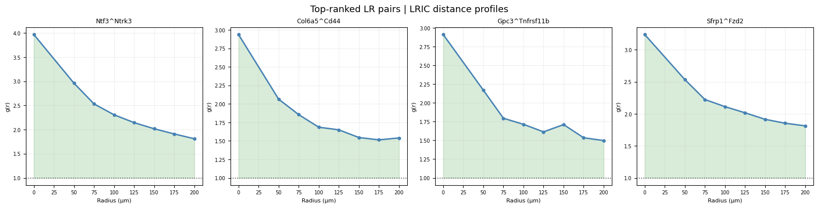
Distance profiles for top-ranked pairs

TOP_N = 4

top = pair_scores.head(TOP_N)["pair"].tolist()

fig, axes = plt.subplots(1, TOP_N, figsize=(4 * TOP_N, 4), layout="constrained")
for ax, pair in zip(axes.flat, top):
    idx = ag["pair_names"].index(pair)
    g   = ag["lric"][:, idx]

    ax.plot(ag["radii"], g, lw=2, marker="o", ms=4, color="steelblue")
    ax.axhline(1, linestyle=":", color="0.3", lw=1.2)
    ax.fill_between(ag["radii"], 1, g, where=g > 1, alpha=0.15, color="green")
    ax.fill_between(ag["radii"], g, 1, where=g < 1, alpha=0.15, color="red")
    ax.set_title(pair, fontsize=9)
    ax.set_xlabel("Radius (µm)", fontsize=8)
    ax.set_ylabel("g(r)", fontsize=8)
    ax.grid(alpha=0.2); ax.tick_params(labelsize=7)

fig.suptitle("Top-ranked LR pairs | LRIC distance profiles", fontsize=13)
plt.show()

LRIC Cell-Type Informed for Directed Interactions

The cell-type-informed mode splits cells into sender and receiver populations by cell-type annotation and computes g(r) for every directed (sender → receiver) pair, weighted by the LR expression.

This answers a more specific question:

For the specific interaction sender cell type X expressing ligand L → receiver cell type Y expressing receptor R, is the LR-weighted spatial co-enrichment at distance r higher than expected?

Key advantage over cross-PCF: the expression weighting means g(r) > 1 can only be driven by cells that express the relevant ligand/receptor.

li.mt.lric(
    adata,
    resource=resource,
    groupby="cell_type",
    spatial_key="X_spatial_coords",
    max_radius=200,
    radius_step=annulus_width,
    annulus_width=annulus_width,
    min_cells=50,
    min_expressing=20,
    use_raw=False,
    key_added="lric_ct", #results will be saved under this label in adata.uns
    verbose=True,
)

Using provided `resource`.

Cross-PCF vs LRIC: Does expression add information?

Cross-PCF captures spatial structure. If LRIC tracks cross-PCF closely, the LR pair’s signal is mostly explained by where the two cell types happen to be. If LRIC exceeds cross-PCF, the expression weighting is amplifying the signal: cells that express the ligand/receptor are not distributed randomly within their cell type but they cluster near each other.

We compare cross-PCF, agnostic LRIC, and CT-specific LRIC for Tac2→Tacr3 (tachykinin neuropeptide signalling) on the GABAergic → glutamatergic axis.

snd, rcv = "GABAergic neuron", "glutamatergic neuron"
ligand, receptor =  "Tac2", "Tacr3"

lric_ct = adata.uns["lric_ct"]
lr_pair = next(p for p in lric_ct["pair_names"] if ligand in p and receptor in p)

# extract g(r) curves for the three views
r_c  = np.asarray(cpcf["radii"], dtype=float)
g_c  = np.asarray(cpcf["results"].get((snd, rcv), np.full_like(r_c, np.nan)), dtype=float)

p_ag = ag["pair_names"].index(lr_pair)
r_ag = np.asarray(ag["radii"], dtype=float)
g_ag = np.asarray(ag["lric"][:, p_ag], dtype=float)

p_ct = lric_ct["pair_names"].index(lr_pair)
r_ct = np.asarray(lric_ct["radii"], dtype=float)
g_ct = np.asarray(lric_ct["results"][(snd, rcv)][:, p_ct], dtype=float)

plot_pair(
    snd, rcv,
    {"cross-PCF": (r_c, g_c), "agnostic LRIC": (r_ag, g_ag), "CT-specific LRIC": (r_ct, g_ct)},
    colors={"cross-PCF": "0.5", "agnostic LRIC": "steelblue", "CT-specific LRIC": "tab:red"},
    title=f"{snd}  ·  {ligand} → {receptor}  ·  {rcv}",
    ligand=ligand, receptor=receptor,
)

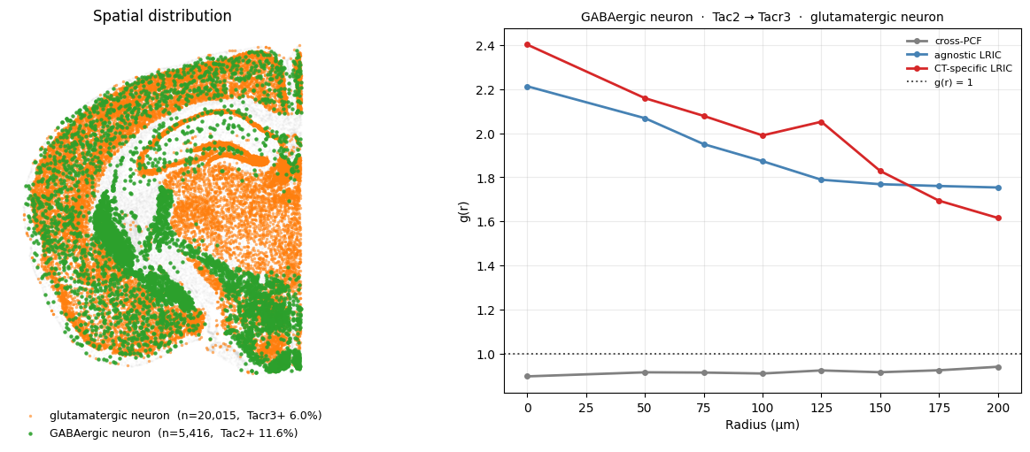
We notice that CT-specific LRIC (red) peaks above the cross-PCF (grey) at short distances. The Tac2/Tacr3 expression pattern reinforces the spatial proximity signal: GABAergic cells that express Tac2 tend to be found near glutamatergic cells that express Tacr3, beyond what the overall cell-type co-localisation would predict.

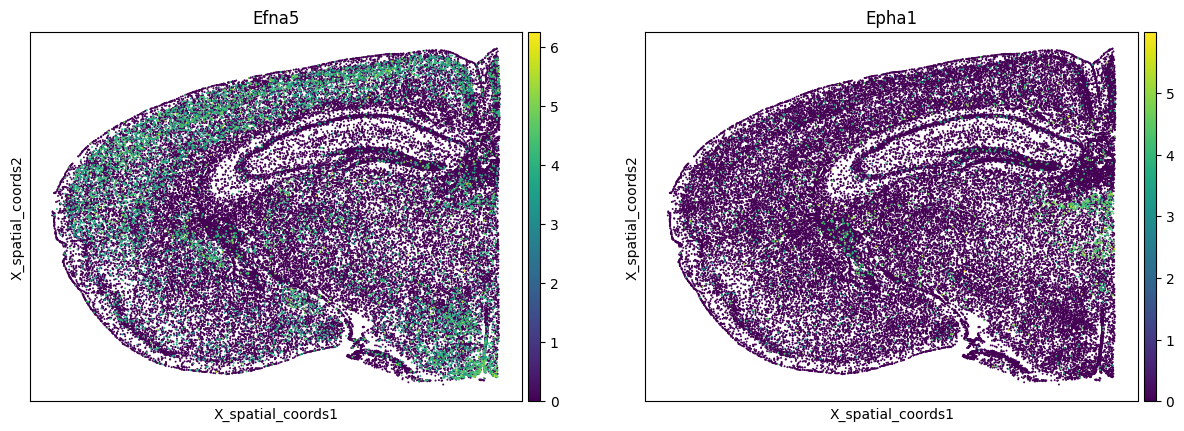
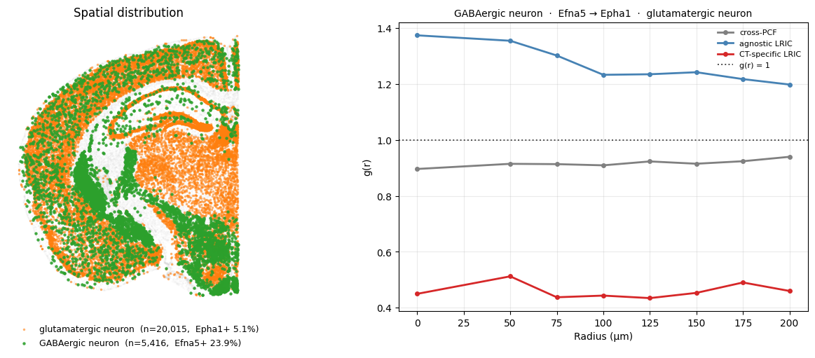
In contrast, Efna5-expressing GABAergic and Epha1-expressing glutamatergic neurons show the opposite pattern. Although the two cell types are broadly co-distributed (cross-PCF ≈ 1), the CT-specific LRIC drops below 1: cells that express these ephrin partners are specifically less likely to be near one another than the overall cell-type co-localisation would suggest.

snd, rcv = "GABAergic neuron", "glutamatergic neuron"
ligand, receptor =  "Efna5", "Epha1"

lric_ct = adata.uns["lric_ct"]
lr_pair = next(p for p in lric_ct["pair_names"] if ligand in p and receptor in p)

# extract g(r) curves for the three views
r_c  = np.asarray(cpcf["radii"], dtype=float)
g_c  = np.asarray(cpcf["results"].get((snd, rcv), np.full_like(r_c, np.nan)), dtype=float)

p_ag = ag["pair_names"].index(lr_pair)
r_ag = np.asarray(ag["radii"], dtype=float)
g_ag = np.asarray(ag["lric"][:, p_ag], dtype=float)

p_ct = lric_ct["pair_names"].index(lr_pair)
r_ct = np.asarray(lric_ct["radii"], dtype=float)
g_ct = np.asarray(lric_ct["results"][(snd, rcv)][:, p_ct], dtype=float)

plot_pair(
    snd, rcv,
    {"cross-PCF": (r_c, g_c), "agnostic LRIC": (r_ag, g_ag), "CT-specific LRIC": (r_ct, g_ct)},
    colors={"cross-PCF": "0.5", "agnostic LRIC": "steelblue", "CT-specific LRIC": "tab:red"},
    title=f"{snd}  ·  {ligand} → {receptor}  ·  {rcv}",
    ligand=ligand, receptor=receptor,
)

sc.pl.embedding(
    adata,
    basis="X_spatial_coords",
    color=[ligand, receptor],
    s=8,
    use_raw=False
)

---